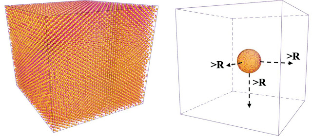
Figure. 1. Simulation box for bulk (left) and nano (right) systems.
In Ref. [1], we discussed the theoretical principles for correcting the nano-size effect when modeling the pair distribution function (PDF). The fundamental idea is to bring back the uncorrelated pairings in between atoms belong to different nanoparticles, based on the assumption of random distribution of nanoparticles in system. Such uncorrelated pairings will then be added to the partial PDF’s calculated explicitly from the structural model in simulation box, as presented in the right of the picture shown above. The kernel mathematical expression in Ref. [1] is reproduced as follows,
\[G(r) = \sum_{i,j}c_ic_jf_if_j[\frac{\rho^{RMC}}{\rho}g_{ij}^{RMC}(r) + U(r) - 1]\]where the meaning of all symbols can be found in Ref. [1] and we won’t reproduce them all here. Instead, we are going to focus on the term \(g_{ij}^{RMC}(r)\) which represents the partial PDF’s calculated explicitly from the simulation box and \(U(r)\) which represents the uncorrelated correlation term. What we are going to discuss here is how to bring these two terms together so that they can be calculated in a compact manner when coded in, e.g., RMCProfile package.
First, \(g_{ij}^{RMC}(r)\) can be further written as,
\[g_{ij}^{RMC}(r) = \frac{n_{ij}}{4\pi r^2dr\rho_j} = \frac{\frac{hist_{ij}}{n_i}}{4\pi r^2dr\frac{n_j}{Vol}} = \frac{hist_{ij}}{4\pi r^2dr\frac{n_i\cdot n_j}{Vol}}\]where \(hist_{ij}\) represents the histogram of pairings between atoms of type \(i\) and \(j\) in system. Basically, it is just the number of pairs between atoms of type \(i\) and \(j\) that fall into specific distance bins. \(Vol\) represents the ‘overall’ volume for calculating the partial number density \(\rho_j\). However, if \(Vol\) in the equation represents the overall volume of the simulation box (where we have void space, to get rid of periodic boundary condition), we then have to bring in an extra correction factor so that the partial number density can be calculated properly. To this point, the factor \(\rho^{RMC}/\rho\) can be introduced, where \(\rho^{RMC}\) and \(\rho\) refers to the overall number density calculated with and without void space in the simulation box, respectively. If we multiple this factor the $Vol$, the effective volume then can be obtained, in which case the equation above just becomes,
\[g_{ij}^{RMC}(r) = \frac{hist_{ij}}{4\pi r^2dr\frac{n_i\cdot n_j}{Vol^{eff}}} = \frac{\rho^{RMC}}{\rho}\frac{hist_{ij}}{4\pi r^2dr\frac{n_i\cdot n_j}{Vol}}\]Next, we focus on the \(U(r)\) term – when coding in such a correction term, we want to do it in a clean way and thus will try to calculate the ‘histogram’ corresponding to the correction term, so that the correction can be applied at the initialization stage and we don’t need to worry about it anymore when calculating the overall PDF and all the other relevant quantities in the program. To do this, we first write,
\[\frac{\rho^{RMC}}{\rho}g_{ij}^{RMC}(r) + U(r) = \frac{\rho^{RMC}}{\rho}\frac{hist_{ij}}{4\pi r^2dr\frac{n_i\cdot n_j}{Vol}} + \frac{U(r)4\pi r^2dr\frac{n_i\cdot n_j}{Vol}}{4\pi r^2dr\frac{n_i\cdot n_j}{Vol}}\]Pulling all the factors out, we will arrive at,
\[\begin{equation}\begin{aligned}\frac{\rho^{RMC}}{\rho}g_{ij}^{RMC}(r) + U(r) & = \frac{\rho^{RMC}}{\rho}\frac{1}{4\pi r^2dr\frac{n_i\cdot n_j}{Vol}}[hist_{ij} + \frac{\rho}{\rho^{RMC}}U(r)4\pi r^2dr\frac{n_i\cdot n_j}{Vol}]\\ & = \frac{\rho^{RMC}}{\rho}\frac{1}{4\pi r^2dr\frac{n_i\cdot n_j}{Vol}}[hist_{ij} + \frac{\rho}{n_{all}/Vol}U(r)4\pi r^2dr\frac{n_i\cdot n_j}{Vol}]\\ & = \frac{\rho^{RMC}}{\rho}\frac{1}{4\pi r^2dr\frac{n_i\cdot n_j}{Vol}}[hist_{ij} + \rho U(r)4\pi r^2dr\frac{n_i\cdot n_j}{n_{all}}]\end{aligned}\nonumber\end{equation}\]where the second term in the square bracket is the effective histogram corresponding to the uncorrelated pairings, which then can be added to the partial PDF’s at the initialization stage.
References
[1] Y. Zhang, et al., J. Appl. Cryst. (2019). 52, 1035-1042.