Taking the \(Y_4^3\) function as the example, the full mathematical form of the function is,
\[Y_4^3 = \frac{3}{4}\sqrt{\frac{35}{\pi}}sin^3\theta cos\theta cos(3\phi)\]To visualize the function, we first need to make it clear what we are trying to visualize. First, physically, this functions gives the distribution of, e.g., the electron density, as the function of the polar angle \(\theta\) and the azimuthal angle \(\phi\) – here it should be noted that it is actually the square of the function that gives the actual density but not the function value itself. Second, the distribution is only about the angular part of the distribution – in another word, the radial part of the distribution is not of a concern here with the spherical harmonics functions. Given a certain combo of \(\theta\) and \(\phi\) values, we can a value of the function – again, this is associated with, e.g., the electron density. But before squaring, the value can be positive or negative, representing the phase of the wavefunction. In 3D space, when we try to visualize the function, we get a series of \(\theta\) and \(\phi\) angles and for each of the combo of \(\theta\) and \(\phi\), we obtain a value which will then be taken as the radius value so to give a coordinate in the 3D space, i.e., \((r, \theta, \phi)\).
Down below is the 3D visualization following such a scheme (with Mathematica), for the \(Y_4^3\) function presented above. The red color is for the positive lobe and the cyan color is for the negative lobe.
In[]:= \[CapitalPsi][\[Theta]_, \[Phi]_] := Sin[\[Theta]]^3*Cos[\[Theta]]*Cos[3*\[Phi]]
 plot3D = SphericalPlot3D[
    Abs[\[CapitalPsi][\[Theta], \[Phi]]], {\[Theta], 0, \[Pi]}, {\[Phi], 0, 2 \[Pi]},
    ColorFunction -> Function[{x, y, z, \[Theta], \[Phi], r}, If[\[CapitalPsi][\[Theta], \[Phi]] > 0, Red, Cyan]],
    ColorFunctionScaling -> False,
    Mesh -> None, PlotPoints -> 50, PlotRange -> All,
    Boxed -> False, Axes -> False,
    Lighting -> "Neutral"
   ]
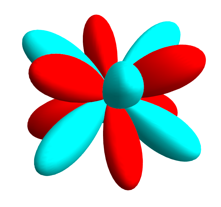
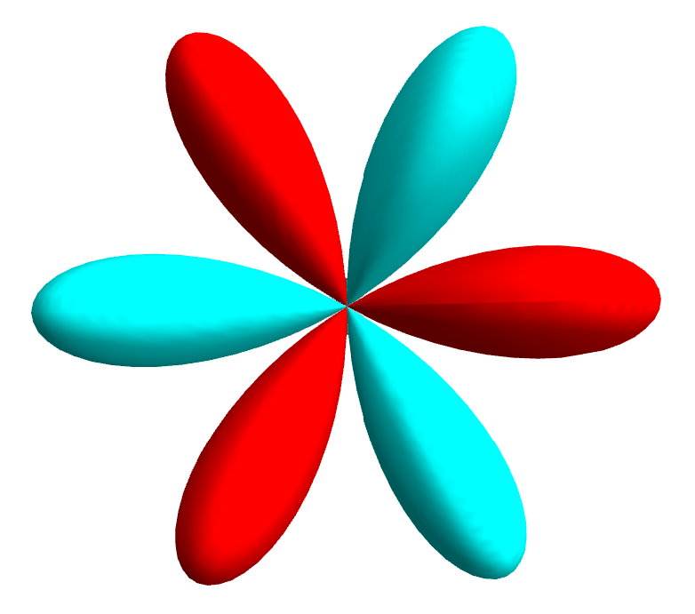
Viewing it from the top, we can clearly see the 6 lobes along the \(\phi\) dimension, and this is a typical shape of the \(g\)-wave Fermi surface.
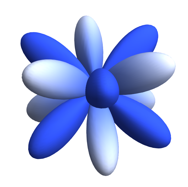
To showcase the gradual change of the function value, we can use other color functions, e.g.,
In[]:= \[CapitalPsi][\[Theta]_, \[Phi]_] := Sin[\[Theta]]^3*Cos[\[Theta]]*Cos[3*\[Phi]]
 plot3D = SphericalPlot3D[
    Abs[\[CapitalPsi][\[Theta], \[Phi]]], {\[Theta], 0, \[Pi]}, {\[Phi], 0, 2 \[Pi]},
    ColorFunction -> Function[{x, y, z, \[Theta], \[Phi], r}, ColorData["TemperatureMap"][\[CapitalPsi][\[Theta], \[Phi]]]],
    ColorFunctionScaling -> False,
    Mesh -> None, PlotPoints -> 50, PlotRange -> All,
    Boxed -> False, Axes -> False,
    Lighting -> "Neutral"
   ]
N.B. In Mathematica, to get a full list of the available color functions, we can do,
In[]:= ColorData["Gradients"]
Out[]= {"AlpineColors", "Aquamarine", "ArmyColors", "AtlanticColors", "AuroraColors", "AvocadoColors", "BeachColors", "BlueGreenYellow", "BrassTones", "BrightBands", "BrownCyanTones", "CandyColors", "CherryTones", "CMYKColors", "CoffeeTones", "DarkBands", "DarkRainbow", "DarkTerrain", "DeepSeaColors", "FallColors", "FruitPunchColors", "FuchsiaTones", "GrayTones", "GrayYellowTones", "GreenBrownTerrain", "GreenPinkTones", "IslandColors", "LakeColors", "LightTemperatureMap", "LightTerrain", "MintColors", "NeonColors", "Pastel", "PearlColors", "PigeonTones", "PlumColors", "Rainbow", "RedBlueTones", "RedGreenSplit", "RoseColors", "RustTones", "SandyTerrain", "SiennaTones", "SolarColors", "SouthwestColors", "StarryNightColors", "SunsetColors", "TemperatureMap", "ThermometerColors", "ValentineTones", "WatermelonColors"}
The full version of the Mathematica notebook can be found in Ref. [1].