This post notes down the understanding of several typical sampling algorithms, including the inverse transform sampling, the rejectin sampling and Markov Chain Monte Carlo sampling. I am not going to cover the nitty-gritty details but just to note down some of what I think as critical points benefiting the understanding of the algorithms.

Inverse transform sampling

inverse_transform

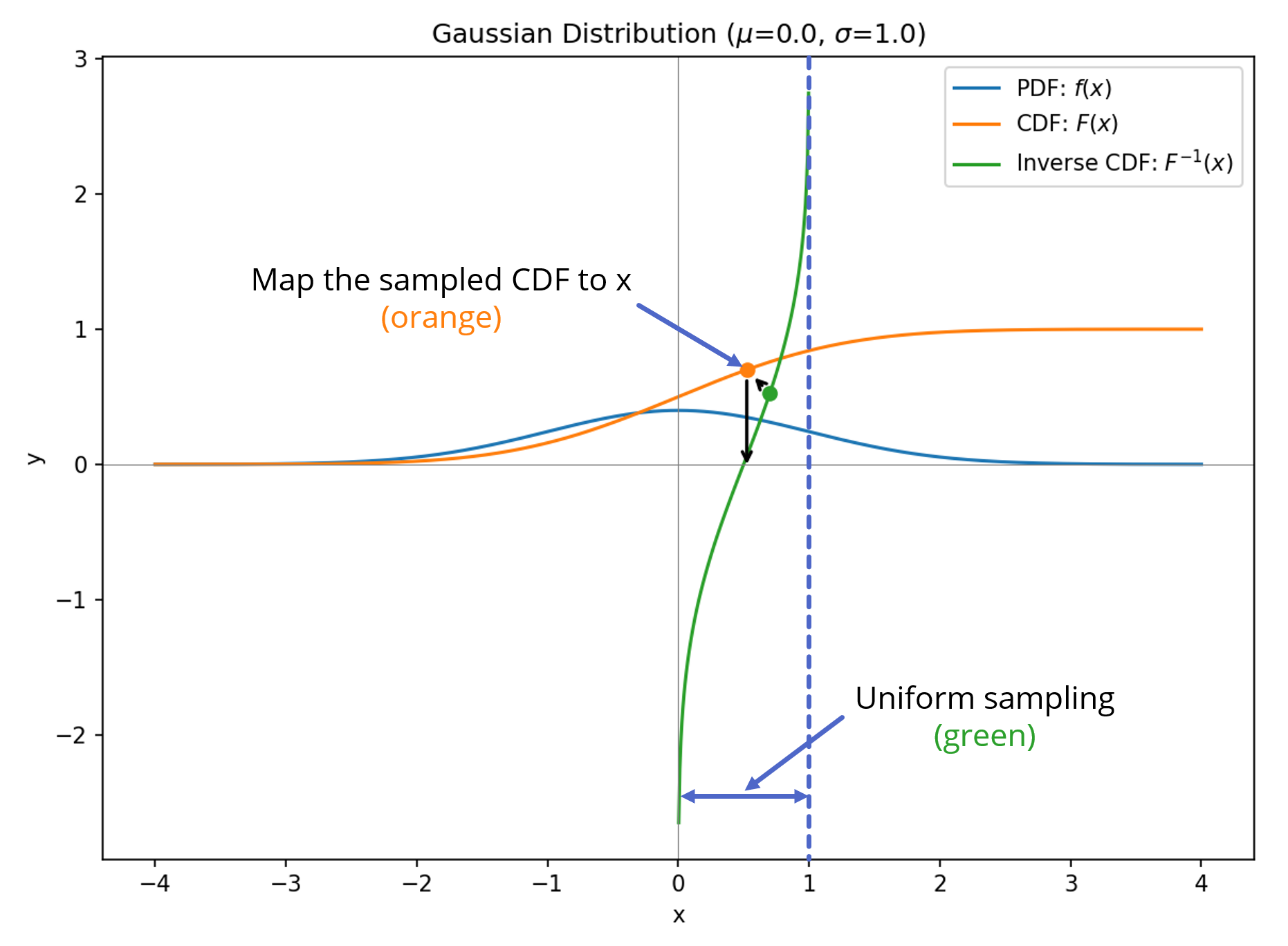
It can be proved by sampling along the x-axis uniformly, the resulted $F^{-1}(U)$ follows the same distribution as the original one, i.e., $X = F^{-1}(U)$ has the same Cumulative Distribution function (CDF) as $F(x)$. The core fact is this: if $U$ is uniform on $(0,1)$ and we define $X = F^{-1}(U)$, then $X$ has exactly the CDF $F(x)$ — and therefore the PDF $f(x) = F'(x)$.
\[P(X \le x) = P(F^{-1}(U) \le x)\]
Since $F$ is monotonically increasing, you can apply $F$ to both sides of the inequality without flipping it:
\[= P(U \le F(x))\]
But $U$ is uniform on $(0,1)$, so $P(U \le u) = u$ for any $u \in [0,1]$. Plugging in $u = F(x)$:
\[= F(x)\]
So $P(X \le x) = F(x)$ — which is by definition what it means for $X$ to have CDF $F$. That’s the whole proof. No calculus needed, just “apply the monotone function $F$ to both sides.”
Since $F'(x) = f(x) = dy/dx$, if we sample $y$ uniformly, the steeper $f(x)$ is, the narrower $x$ range we would end up with. Then as compared to the flat region of the $F(x)$ function, the $x$ values in the narrower regions have more chances to be picked/sampled, i.e., the inverse transform sampling indeed samples following the $f(x)$ distribution.

Rejection sampling

rejection

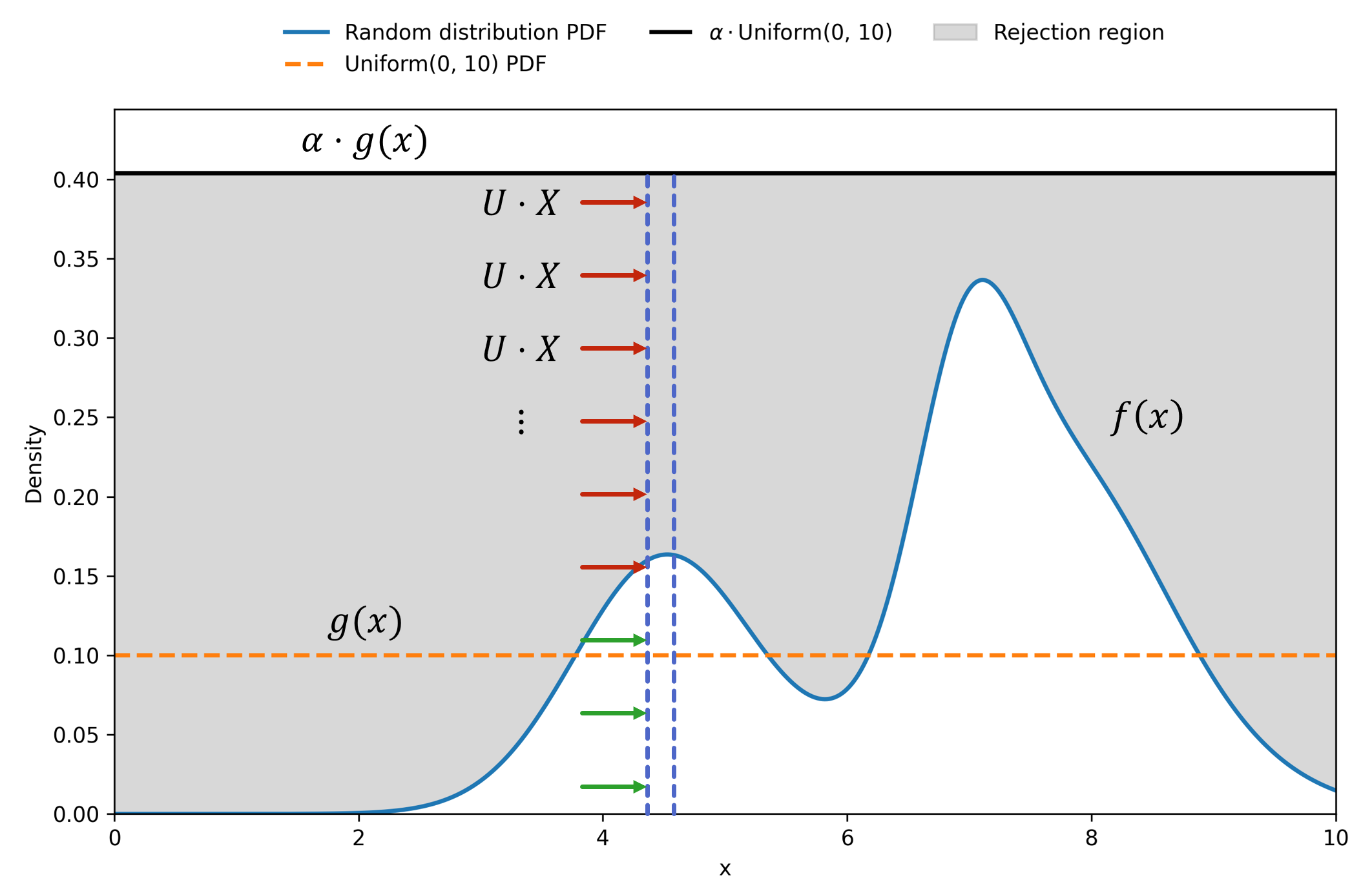
$g(x) \Rightarrow$ a picked distribution
$\alpha\cdot g(x) \Rightarrow \alpha$ picked so that we have $\alpha\cdot g(x) > f(x), \forall x$
$X \Rightarrow$ sampled from $g(x)$
$U \Rightarrow$ sampled from $\text{Uniform}(0, 1)$
If $U\cdot X < f(x) \Rightarrow$ accept
Else $\Rightarrow$ reject & repeat

Some notes,

The acceptance probability is determined by the height of $f(x)$ at $X$ and therefore the accepted samples $X$’s follow the $f(x)$ distribution.
Sampling of $X$ is biased by $g(x)$ but the acceptance rate is dominated by $f(x)$. Therefore, the accpeted sampling follows the $f(x)$ distribution. Imagine we are not using a uniform distribution $g(x)$ for the initial sampling and we may have the PDF $g(x)$ having large values in certain regions of $x$. Sampling will then be biased towards those regions. However, the more it is biased towards those regions, the less probable that the sampling in those regions will be accepted, since the proportion of the rejected region along the vertical direction (see the region bounded by the dashed blue lines in the figure and the shaded region inside the bounded box) is larger.

Markov Chain Monte Carlo

Detailed notes about the Markov Chain Monte Carlo (MCMC) sampling algorithm can be found in my earlier post here. Here below I am putting down some side notes about the algorithm.

mcmc

Download scrpts for creating the figures above here.

Sampling is dominated by the probability density function (PDF), or put the other way round, a proper sampling scheme should be the one to yield a distribution that follows the target PDF.
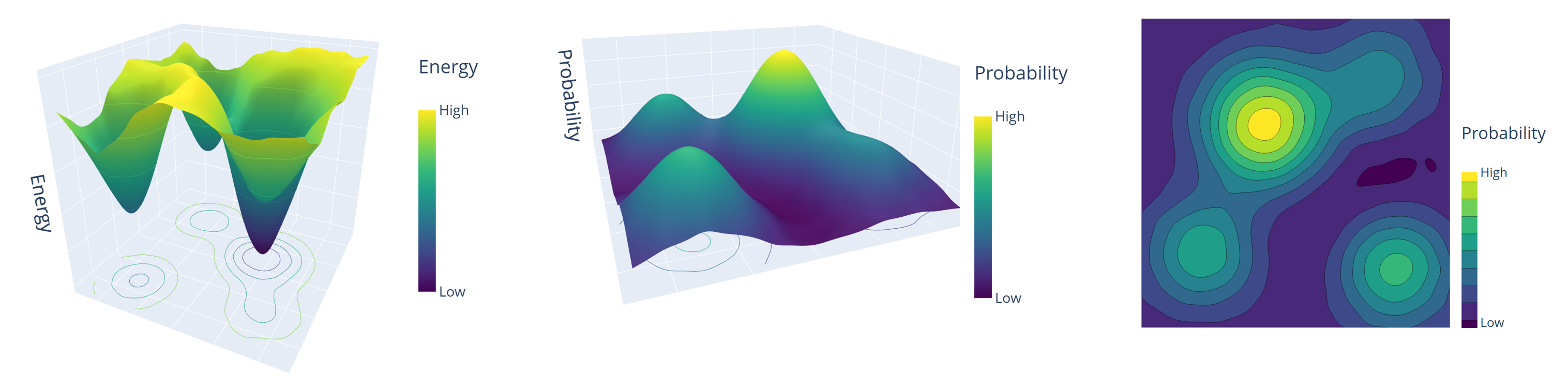
MCMC algorithm follows the same principle, and the sampling is dominated by the PDF shown in the middle panel above (the right panel shows the corresponding contour plot).
Physically, for systems following Boltzmann distribution, the PDF is determined by the energy landscape, $f(x) = \frac{1}{\mathcal{Z}}e^{-\frac{E(x)}{k_BT}}$, where the partition function $\mathcal{Z}$ is usually unknown in practice.

N.B. $x$ here is a high dimensional vector in the configuration space and here we are using 2D for the demo purpose.
Running the MCMC chain, the system will finally converge to the PDF distribution, i.e., it is converging to any single state but instead to a distribution. This means that if we keep running the chain after convergence, the system state will still fluctuate, but the resulted configurations along the chain altogether will follow the PDF distribution. If the system has a well-defined global minimum like the 2D example shown here, since the PDF function has a large value at the global minimum (when I say ‘minimum’, I am referring to the energy landscape), the sampled states will have a very high probability to end up in that region.