The image was generated with Gemini with the prompt of ‘Generate an image as an abstract showcase for the variational autoencoder. Use the Ghibli style’.

1. General Introduction

A Variational Autoencoder (VAE) is a generative model that represents data through a probabilistic latent space, allowing new data to be synthesized by sampling from that latent space and decoding the samples [1, 2]. This distinguishes it from a conventional (non-variational) autoencoder, which learns a deterministic mapping from an input to a single latent code and back to a reconstruction, with no sampling operation involved at any stage of normal use: encoding is \(z = f(x)\) and decoding is \(\hat{x} = g(z)\), both fixed functions.

The training objective of a conventional autoencoder minimizes reconstruction error alone (e.g., \(\|x - g(f(x))\|^2\)), without imposing any structure on the latent space. As a result, most points in that latent space are never visited during training, and decoding an arbitrarily chosen latent point typically produces unstructured, meaningless output – the autoencoder’s latent space is, in general, not sample-able.

For a non-variational autoencoder, the non sample-able latent space is not a problem since we are not supposed to sample the latent space anyways – the whole purpose of a conventional autoencoder is to compress the input effectively into the latent space from which then the input can be re-generated reliably. In another word, the conventional autoencoder is not supposed to be a generative tool with which we can generate some new samples given the trained network. To have such generative autoencoder, a VAE comes to the spot by changing the training scheme in two ways:

1. The encoder outputs the parameters of a probability distribution over the latent space for each input, rather than a single latent code.
2. The aggregate of these latent distributions is explicitly regularized, during training, toward a fixed and known prior distribution – typically a standard multivariate normal distribution, \(\mathcal{N}(0, I)\).

Because each input is mapped to a distribution (a “cloud” of plausible latent values) rather than a single point, and because these clouds are collectively pushed toward the prior, the decoder is exposed to – and learns to handle – a densely and continuously populated region of latent space. This is what makes it possible, once training is complete, to bypass the encoder entirely, draw a fresh latent sample directly from the known prior, and decode it into a novel, plausible output. This generative capability is the central practical benefit of the VAE framework over a conventional autoencoder.

It is also important to note that neither the encoder nor the decoder produces a data point directly – each network predicts the parameters of a distribution, and the corresponding data point is (in principle) a sample drawn from that distribution:

• The encoder produces the parameters (mean and variance) of a distribution over the latent space, \(q_\phi(z \mid x)\), from which a latent vector \(z\) is sampled.

• The decoder produces the parameters of a distribution over the output space, \(p_\theta(x \mid z)\) – for example, a mean vector under a Gaussian likelihood, or a set of per-element probabilities under a Bernoulli likelihood – from which the output is, in principle, itself sampled.

  
  

  For the Bernoulli case, here is an example to showcase how it works. For instance, suppose the decoder predicts that a pixel has an 80% chance of being white and a 20% chance of being black. Then, to generate the value for the pixel, we can generate a random number between 0 and 1. If the generated number is greater than 0.2, the pixel is sampled as white; otherwise, it is black.

In practice, if we are dealing with continuous generation problems (e.g., generating RGB-color images where each pixel has continous values), we will be using the Gaussian distribution for the output generation. In this case, the out sampling step is usually reporting the mean of the output distribution, since the meaningful variability for generation has already been introduced by sampling \(z\); sampling again at the output stage typically adds little beyond low-level noise. This matters mathematically, because the reconstruction term of the training objective is derived directly from the assumed form of this output distribution (Section 2.2).

The end-to-end pipeline of a VAE can be summarized in the following diagram,

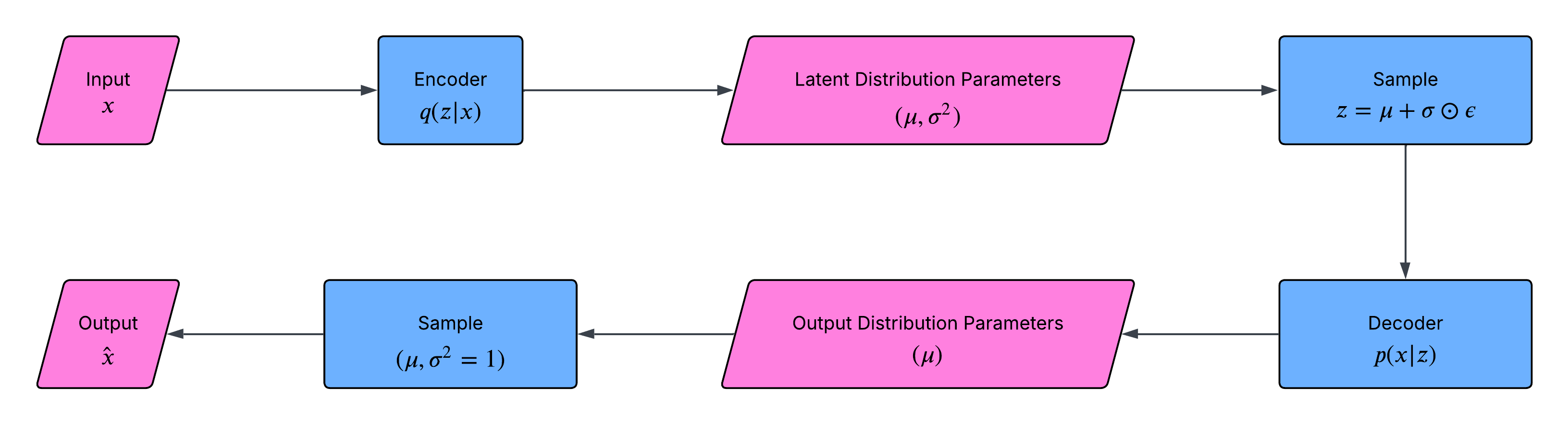
N.B. The \(\sigma^2 = 1\) in the output sampling step is an arbitrarily chosen value, as a hyperparameter (see the discussion above for the justification of doing so).

2. Some Maths

This section presents the mathematical foundations of the variational autoencoder framework: the derivation of the Evidence Lower Bound (ELBO), the derivation of the training loss under two different assumed output likelihoods, and a list of supporting background topics.

2.1 Derivation of the Evidence Lower Bound (ELBO)

Consider data \(x\) assumed to be generated by an unobserved latent variable \(z\) through a generative process \(p_\theta(x\mid z)\), with prior distribution \(p(z) = \mathcal{N}(0, I)\). The marginal likelihood of the data is

This integral is intractable in general, since the decoder \(p_\theta(x\mid z)\) is a nonlinear neural network and we cannot enumerate all \(z\)’s. To circumvent this, an approximate posterior distribution \(q_\phi(z\mid x)\) (implemented by the encoder network) is introduced and used to derive a tractable lower bound on \(\log p_\theta(x)\).

Consider the Kullback-Leibler (KL) divergence between the approximate posterior \(q_\phi(z\mid x)\) and the true, intractable posterior \(p_\theta(z\mid x)\),

By Bayes’ rule, \(p_\theta(z\mid x) = \dfrac{p_\theta(x\mid z)\,p(z)}{p_\theta(x)}\). Substituting this into the KL divergence formulation, we have,

Since \(\log p_\theta(x)\) does not depend on \(z\), it can be moved outside the expectation:

Rearranging:

Because KL divergence is always non-negative, the first term – the Evidence Lower Bound (ELBO) – constitutes a lower bound on the marginal log-likelihood:

Since the true posterior \(p_\theta(z\mid x)\) is unavailable, the ELBO is maximized in its place; doing so simultaneously increases \(\log p_\theta(x)\) and drives \(q_\phi(z\mid x)\) toward the true posterior [1, 2].

Remark on covariance structure. Both \(q_\phi(z\mid x)\) (the encoder’s latent distribution) and, when a Gaussian output likelihood is used, \(p_\theta(x\mid z)\) (the decoder’s output distribution) are multivariate Gaussian distributions. In standard VAE formulations, the different dimensions of each distribution are assumed statistically independent given the conditioning variable, so that the covariance matrix is restricted to be diagonal (or, for the output likelihood, isotropic with a single shared scalar variance). This assumption reduces the number of parameters that must be predicted from \(O(d^2)\) to \(O(d)\), allows sampling to be performed independently per dimension (Section 1.1), and – as shown in Section 2.2.2 – allows the KL divergence term to be written in closed form as a sum of independent per-dimension terms [4, 5].

2.2 Loss Function Derivation

The ELBO consists of two terms that are optimized jointly:

Training maximizes \(\mathcal{L}\), equivalently minimizing \(-\mathcal{L}\) as a loss.

The reconstruction term is an expectation over \(q_\phi(z\mid x)\) with no closed form (an explicit algebraic formula), since the decoder is a nonlinear network; it is approximated with a single Monte Carlo sample per training step. Direct sampling of \(z\) is not differentiable with respect to \(\phi\), so the reparameterization trick is used [1, 2]: the sample is rewritten as a deterministic, differentiable function of an independent noise variable,

with \(\odot\) denoting the elementwise (Hadamard) product. Since \(\mu\) and \(\sigma\) (outputs of the encoder) enter through a differentiable path and all stochasticity is isolated in \(\epsilon\), gradients with respect to \(\phi\) can be computed normally. With one such sample, the reconstruction term is approximated as

i.e., by decoding the single sampled \(z\) and evaluating the resulting output likelihood. Its exact form depends on the assumed output distribution.

2.2.1 Reconstruction Term

Gaussian Output Distribution

Assume a Gaussian output likelihood with fixed, isotropic variance \(\sigma_x^2\) (a hyperparameter, not predicted by the network),

For a single scalar element (e.g., one pixel),

Under the diagonal (here, isotropic) covariance assumption, elements are conditionally independent given \(z\), so the joint log-likelihood over all \(n\) elements sums (the joint likelihood should be multiplicative but the log-likelihood turns that into summation),

Negating, to obtain a quantity to be minimized:

Because \(\sigma_x^2\) is fixed rather than predicted by the network, the first term is a constant with no dependence on \(\theta\) or \(\phi\), and the coefficient \(1/(2\sigma_x^2)\) is a fixed positive scalar that does not change the location of the minimum. Both can be dropped:

That is, the negative log-likelihood under a fixed-variance Gaussian output distribution reduces to the squared error between the input and the decoder’s mean output – the Mean Squared Error (MSE) loss. This mirrors the classical result that least-squares regression is the maximum-likelihood estimator under an assumption of homoscedastic Gaussian noise.

Homoscedastic: multiple observations possess the same variance.

Note: if the decoder instead predicts a per-element variance \(\sigma_{x,\theta}^2(z)\) in addition to the mean, the \(\log(2\pi\sigma_x^2)\) term becomes \(\theta\)-dependent and cannot be dropped; the loss then takes the form of a full heteroscedastic Gaussian negative log-likelihood. This variant is less common in practice, in part because the predicted variance can degenerate toward zero during optimization. Here follows is a bit more illustration regarding such a failure mode. Suppose, for some training point, the network manages to get its mean prediction \(\hat{x}_i\) very close to the true value \(x_i\) – so the residual \((x_i - \hat{x}_i)^2\) is small. Once that residual is small, we can take look at what happens as \(\sigma_{x,i}^2 \to 0\):

• The quadratic term \(\dfrac{(x_i-\hat{x}_i)^2}{2\sigma_{x,i}^2}\) stays bounded (small numerator divided by small denominator, but the numerator is already small before dividing, so this term doesn’t necessarily explode – it depends on how fast the residual shrinks relative to \(\sigma^2\)).

• The log term \(\dfrac{1}{2}\log(2\pi\sigma_{x,i}^2)\) marches toward \(-\infty\) as \(\sigma_{x,i}^2\to 0\), with no floor.

So the network discovers a cheap trick: for any point where it’s already fitting reasonably well, it can keep shrinking \(\sigma_{x,i}^2\) toward zero, and the log term keeps driving the loss down toward \(-\infty\), unboundedly. In another word, the networks sees a shortcut to reduce the loss by reducing the variance, therefore losing the ‘interest’ in predicting the mean value more accurately.

Bernoulli Output Distribution

For binary or \([0,1]\)-normalized data, a Bernoulli output likelihood is commonly assumed instead. Each element \(x_i \in \{0,1\}\) is modeled as

where \(\hat{x}_i(z)\) is the decoder’s output, typically obtained via a sigmoid activation. Unlike the Gaussian case, the Bernoulli distribution has a single parameter that determines both its mean and its variance, so no separate variance term needs to be introduced. The probability mass function is

Taking the logarithm and summing over all \(n\) elements (again assuming conditional independence given \(z\)):

Negating gives the loss directly, with no constant terms to discard:

This expression is exactly the Binary Cross-Entropy (BCE) loss, summed over all elements. In practice this quantity is computed from the decoder’s pre-sigmoid logits using a numerically stable, fused implementation, to avoid overflow as \(\hat{p}_i \to 0\) or \(\hat{p}_i \to 1\). Here below are presented the details.

Why the naive computation is unstable. The decoder’s final layer typically produces an unbounded logit \(\ell_i \in (-\infty,\infty)\), with \(\hat p_i = \sigma(\ell_i) = 1/(1+e^{-\ell_i})\). If \(\hat p_i\) is computed first and then substituted directly into the BCE formula, two floating-point failure modes arise for extreme values of \(\ell_i\):

• If \(\ell_i\) is very negative, \(\hat p_i\) underflows to exactly \(0.0\) in floating-point representation. If the true label is \(x_i=1\), the loss contains \(\log(0.0) = -\infty\), and this propagates: finite + (-inf) = -inf for the batch total.
• If \(\hat p_i\) underflows to \(0.0\) while the true label is \(x_i=0\), the corresponding term is \(x_i\log\hat p_i = 0\cdot\log(0.0) = 0\cdot(-\infty)\). Mathematically this term should vanish (the coefficient \(x_i=0\) eliminates it), but IEEE floating-point arithmetic evaluates \(0\times\infty\) as NaN, since the two factors reach their limiting values independently and there is no way to resolve the product consistently from the numerical values alone. The corresponding gradient is equally fragile: \(\dfrac{d}{d\hat p_i}\log\hat p_i = 1/\hat p_i\), which diverges as \(\hat p_i\to 0\) and can itself overflow to inf in floating point before \(\hat p_i\) even reaches exact zero. Once an inf or NaN value enters a gradient tensor, the chain rule propagates it through every downstream computation in the backward pass, and a subsequent optimizer step assigns NaN to the corresponding network weights – from that point on, every forward pass using those weights also produces NaN, so the corruption is not confined to the single offending element.

Derivation of the stable, logits-based formula. Expanding \(\log\hat p_i\) and \(\log(1-\hat p_i)\) directly in terms of the logit \(\ell_i\) removes the need to ever evaluate \(\log\) of a quantity that can round to exactly \(0\) or \(1\). First,

Second, using \(1-\hat p_i = \dfrac{e^{-\ell_i}}{1+e^{-\ell_i}}\),

Substituting both into the BCE expression for a single element and distributing the sign,

This form is already safe for very negative \(\ell_i\), but can still overflow for very large positive \(\ell_i\) if computed as written. Adding and subtracting \(\max(\ell_i,0)\) – an identity verified by checking the cases \(\ell_i\geq 0\) and \(\ell_i<0\) separately – yields a form that is symmetric in \(\ell_i\):

The only exponential term remaining is \(e^{-\vert\ell_i\vert}\), and since \(\vert\ell_i\vert\geq 0\) always, this quantity satisfies \(e^{-\vert\ell_i\vert}\in(0,1]\) regardless of how large \(\ell_i\) becomes in either direction. Consequently \(1+e^{-\vert\ell_i\vert}\in(1,2]\), so the log term is always finite and bounded, and no probability value is ever explicitly computed or passed through a logarithm. This is the formula implemented by fused operations such as binary_cross_entropy_with_logits, operating directly on the decoder’s logits rather than on \(\hat p_i\) itself.

2.2.2 KL Divergence (Regularization) Term

Because both \(q_\phi(z\mid x) = \mathcal{N}(\mu,\Sigma_0)\) and the prior \(p(z) = \mathcal{N}(0,I)\) are multivariate Gaussian distributions, their KL divergence has a closed form and requires no Monte Carlo estimation. The general closed-form KL divergence between two multivariate Gaussians \(\mathcal{N}(\mu_0,\Sigma_0)\) and \(\mathcal{N}(\mu_1,\Sigma_1)\) in \(d\) dimensions is

Setting \(\mu_1=0\), \(\Sigma_1=I\) (the prior) and \(\Sigma_0=\text{diag}(\sigma_1^2,\dots,\sigma_d^2)\) (the diagonal-covariance encoder output, per the remark in Section 2.1), we have,

Substituting all the terms back into the KL divergence yields,

Equivalently, this result follows directly from the fact that a diagonal-covariance multivariate Gaussian factorizes into a product of \(d\) independent univariate Gaussians, \(q_\phi(z\mid x)=\prod_{j=1}^d\mathcal{N}(z_j;\mu_j,\sigma_j^2)\), and the KL divergence between two product distributions equals the sum of the KL divergences of their factors. The univariate KL divergence \(D_{KL}(\mathcal{N}(\mu,\sigma^2)\|\mathcal{N}(0,1))\), obtained by expanding \(\mathbb{E}_q[\log q(z)-\log p(z)]\) and using \(\mathbb{E}_q[z^2]=\mu^2+\sigma^2\) (Section 2.3), reduces to \(\tfrac{1}{2}(\mu^2+\sigma^2-\log\sigma^2-1)\) per dimension, consistent with the multivariate result above [4, 5]. Here below is the presented the detailed derivation,

First, start from the KL divergence definition,

with \(q(z) = \mathcal{N}(\mu,\sigma^2)\) and \(p(z) = \mathcal{N}(0,1)\).

Then we write out both log-densities,

Substituting back into the KL divergence expression yields,

The two \(\log(2\pi)\) pieces combine: \(-\tfrac12\log(2\pi\sigma^2)+\tfrac12\log(2\pi) = -\tfrac12\log\sigma^2\) (since \(\log(2\pi\sigma^2) = \log(2\pi)+\log\sigma^2\), the \(\log(2\pi)\) terms cancel). So:

Finally we take the expectation under \(q\), term by term,

Two expectations need evaluating:

• \(\mathbb{E}_q[(z-\mu)^2]\): this is, by definition, the variance of \(z\) under \(q\) — since \(q=\mathcal{N}(\mu,\sigma^2)\), that variance is exactly \(\sigma^2\).
• \(\mathbb{E}_q[z^2]\): see Section 2.3.

Substituting the results back into the KL divergence, we have,

which reproduces the result from the multi-variate derivation.

Combining the reconstruction and regularization terms, and introducing a weighting coefficient \(\beta\) on the regularization term as in the \(\beta\)-VAE formulation [3], the total per-example training loss is

where \(\mathcal{L}_{\text{reconstruction}}\) is either the squared-error term (Section 2.2.1, Gaussian case) or the binary cross-entropy term (Section 2.2.1, Bernoulli case), depending on the assumed output likelihood. Setting \(\beta=1\) recovers the standard VAE objective; \(\beta>1\) places additional weight on the regularization term, generally at the cost of reconstruction fidelity, and has been associated with more disentangled latent representations [3].

Disentangled latent representation here means the different dimensions in the latent space are determining the image features independently.

2.3 Background Knowledge

Here in this session I am presenting several pieces of mathematical background knowledge for better understanding the story flow presented above.

Bernoulli Distribution

When we have a series of observations, and for each of the obeservations we have binary results, e.g., \(0\) or \(1\), with the probability of \(p(X=0) = p\) and \(p(X=1) = 1 - p\), respectively, such a distribution of observation values is the Bernoulli distribution. The probability mass function (see next bit) can be written in a compact form, as,

Here, \(k\) refers to the possible binary values, e.g., \(0\) for coin head up and \(1\) for coin tail up. \(p\) is the probability of the variable taking \(k = 0\).

Probability Mass Function

The function presented in the previous chunk,

is called the probability mass function, which is the probability distribution of a discrete random variable. For a discrete random variable, the probability for each discrete value can be given directly – by comparison, for continuous random variable, the probability can only be given for a certain range of the variable by integrating the probability density function (PDF) over that region.

Derivation of \(\mathbb{E}[z^2]\)

If we have the random variable \(z\) following the Gaussian distribution, \(z \sim \mathcal{N}(\mu, \sigma^2)\), here we are trying to derive \(\mathbb{E}[z^2]\). First, we have the variance of \(z\) defined as,

Expanding the expression inside the square bracket, we have,

\(\mathbb{E}[z]\) is a constant so can be pulled out from expectation value calculations like \(\mathbb{E\big[2\mathbb{E}[z] \cdot z\big]}\) to have \(\mathbb{E\big[2\mathbb{E}[z] \cdot z\big]} = 2\mathbb{E}[z] \cdot \mathbb{E}[z]\).

Given \(z \sim \mathcal{N}(\mu, \sigma^2)\), we have \(\text{Var}(z) = \sigma^2\), and rearranging the derivation above gives,

The result here is used in Section 2.2.

References

[1] D. P. Kingma and M. Welling, arXiv:1312.6114, 2013.

[2] D. J. Rezende, S. Mohamed, and D. Wierstra, arXiv:1401.4082, 2014.

[3] I. Higgins, L. Matthey, A. Pal, C. Burgess, X. Glorot, M. Botvinick, S. Mohamed, and A. Lerchner, ICLR, 2017.

[4] C. Doersch, arXiv:1606.05908, 2016.

[5] C. M. Bishop, Pattern Recognition and Machine Learning, Springer, 2006.