optimization_header
Image generated with Gemini with the prompt ‘generate an abstract image for my blog post about optimization methods like Newton method, Gauss-Newton, Levenberg-Marquardt, etc,. use the Ghibli style’.

A summary of optimization methods will be presented in the current post, giving an idea about what methods we have, their categories and relations. No details about any methods (derivation, pros and cons, etc.) will be given – I would treat the post as a rough collection, some backbone maths and maybe a map to those methods. I will put some interesting and helpful references wherever relevant.

Direction-First Methods

This is just how I call it and I am not sure what category that people usually call these methods. I am not even sure whether people usually categorize them in this way. Anyhow, I thought all the methods included in the current section first decided the direction to go along, followed by deciding how much to go along the determined direction. Therefore, I chose to call them altogether as ‘direction-first’ methods.

Newton Method

Formulation,

\[\vec{x}_{k + 1} = \vec{x}_{k} - \mathbb{H}(\vec{x}_k)^{-1}\nabla f(\vec{x}_k)\]

In one-dimension, simply we have,

\[x_{k + 1} = x_k - \frac{f'(x_k)}{f''(x_k)}\]

For high dimension, it is just that the first and second derivative (partial) becomes the gradient and the Hessian.

Gauss-Newton Method

Formulation,

\[\begin{align} \mathbb{J}^T\mathbb{J}\vec{\delta} & = -\mathbb{J}^T\vec{r}\\ \vec{\beta}_{k + 1} & = \vec{\beta}_{k} + \vec{\delta} \end{align}\]

\(\vec{\delta}\): steping direction
\(\vec{r} = \vec{y} - f(\vec{x}, \vec{\beta})\): the residual, with \(\vec{y}\) being the observed values and \(f(\vec{x}, \vec{\beta})\) being our model.
\(\mathbb{J}\): the Jacobian, \(J_{ij} = \partial r_i/\partial\beta_j\).

The \(\mathbb{J}^T\mathbb{J}\vec{\delta}\) term in the formulation can be regarded as an approximated version of the Hessian.

BFGS Method

BFGS: Broyden–Fletcher–Goldfarb–Shanno

A method very similar to the Newton method – the inverse Hessian as given in the Newton’s method formulation is replaced with its approximate version, which is evaluated in an iterative manner on-the-fly during the optimization. Formulation will not be presented here – see the Algorithm session on its Wiki page.

The three methods above all require Hessian or the approximated Hessian.

Also, at this point (and the same for several methods below as well, before we talk about the dampening of step), we are taking the suggested direction and step as is without any adjustment of the step size. In practice, this is not what we usually do. Instead, the step size will be adjusted – see the discussion below about step dampening.

Gradient Descent

Simple principle applies here – we just follow whevever the gradient points us to. Formulation,

\[\vec{x}_{k + 1} = \vec{x}_{k} - \nabla f(\vec{x}_k)\]

In one-dimension, simply we have,

\[x_{k + 1} = x_k - f'(x_k)\]

Conjugate Gradient Descent

Variation ofthe gradient descent method. Formulation,

\[\begin{align} \vec{x}_{k + 1} & = \vec{x}_k + \vec{\delta}_k\\ \vec{\delta}_{k + 1} & = -\nabla f(\vec{x}_{k + 1}) + \beta_k\vec{\delta}_k \end{align}\]

starting with \(\vec{\delta}_0 = -\nabla f(\vec{x}_0)\).

The choice of \(\beta_k\) defines the variant. Writing \(\vec{g}_k = \nabla f(\vec{x}_k)\), we have the following variants,

\[\begin{align} \beta_k^{FR} &= \frac{\vec{g}_{k+1}^T \vec{g}_{k+1}}{\vec{g}_k^T \vec{g}_k} && \text{(Fletcher-Reeves)} \\ \beta_k^{PR} &= \frac{\vec{g}_{k+1}^T (\vec{g}_{k+1} - \vec{g}_k)}{\vec{g}_k^T \vec{g}_k} && \text{(Polak-Ribiere)} \\ \beta_k^{HS} &= \frac{\vec{g}_{k+1}^T (\vec{g}_{k+1} - \vec{g}_k)}{\vec{\delta}_k^T (\vec{g}_{k+1} - \vec{g}_k)} && \text{(Hestenes-Stiefel)} \\ \beta_k^{DY} &= \frac{\vec{g}_{k+1}^T \vec{g}_{k+1}}{\vec{\delta}_k^T (\vec{g}_{k+1} - \vec{g}_k)} && \text{(Dai-Yuan)} \end{align}\]

Levenberg-Marquart (LM) Method

This is the standard algorithm for nonlinear least square fittings. It kind of brings together the Gauss-Newton method and the gradient descent method, balancing the stability and speed of convergence between the two – instability for Gauss-Newton and slow convergence for gradient descent. Using the same notation as for Gauss-Newton, we have,

\[\begin{align} (\mathbb{J}^T\mathbb{J} + \lambda\mathbb{D})\vec{\delta} & = -\mathbb{J}^T\vec{r}\\ \vec{\beta}_{k + 1} & = \vec{\beta}_{k} + \vec{\delta} \end{align}\]

\(\lambda\) can be fixed or can be updated during the optimization on-the-fly. Details about the updating method can be found in Ref. [1]. Another useful reference is Ref. [2]. For the matrix \(\mathbb{D}\),

Levernberg: \(\mathbb{D} = \mathbb{I}\)
Marquardt: \(\mathbb{D} = \text{diag}(\mathbb{J}^T\mathbb{J})\)

We haven’t specifically mentioned the dampening yet for adjusting the step size as suggested by various methods presented above. With the LM method, we see the dampening parameter for the first time in the current post – just the \(\lambda\) parameter here. Its dampening role is understandable – it comes as a multiplicative factor in front of the steping size to be solved and therefore a larger value of \(\lambda\) obviously induces stronger dampening over the magnitude of \(\vec{\delta}\).

Step Dampening

The current section, as the title suggested, is all about those methods with the steping direction decided first. For simple optimization problems, those methods mentioned above can be taken directly without adjustment. However, in practice, for optimization problems with complex landscape, we do need to have some adjustments. Varying the step size is a typical approach. Apart from the LM method just above (which by itself contains the dampening term already), all the methods mentioned above can be tweaked a bit to introduce a multuplicative factor in front of the suggested step size. It does not matter whether the steping direction is proposed using Hessian, approximated Hessian or gradient – whichever one, we just plug in a multiplicative factor in front of the suggested steping vector.

Determining the value of the step dampening factor needs some dedicated method and typically, the line search method will be used. Refs. [5-7] both provide very insightful explanation about the method.

Trust Region Method

The whole section above is taking a similar route for the optimization in terms of determining the steping direction first and then we decide how far we want to go along that determined direction, either aggressively or conservatively (controlled by the dampening factor – we call it dampening factor but actually it can be amplifying as well since anyhow it is just a multiplicative factor). The trust region method takes another route for optimization. We first pin down the region and within that region, we write down an approximate version of our function to be optimized. Then we trust that inside the pinned region, the approximation is accurate so that we can perform the optimization using the approximate version – this is why the method is called trust region method. So, in contrast to those direction-first methods, the trust region method is kind of a step-size-first method, i.e., we first decide by how much (the most) we want to move and then within the trial boundary, we decide what direction and the actual step size to take. During the optimization, the radius of the trust region will also be adjusted.

The maths behind the method is a bit involved and I never fully got into it. Ref. [3], though, provides a very nice explanation for the method together with the algorithm design and some Python codes.

Nelder-Mead Method

This is a very interesting method and learning something like this is really a great fun. We select a few points (called simplex) in the parameter space, evaluate our function (to be optimized) value at those points. We order them by their values and pick the worst one – for example, if we want to minimize our function, we just pick the one with the greatest value. Then we want to propose a new position in the parameter space to replace our worst simplex (or in some cases, we may need to move all simplex points except the best one), depending on the position of other simplex and their values. The actual process involves the calculation of the centroid (center of gravity), the reflection point (geometry-wise), the evaluation of function values at the reflection point and the comparison to the best and second best among the simplex. Once we figure out the replacement for the worst point according to the algorithm, we update the simplex points and such a process will continue. This is an over-simplication of the algorithm but I believe it can give us some rough ideas about what is happening with the algorithm. A very nice explanation can be found in Ref. [4].

Graphically, the simplex points travel together in the parameter space while changing its shape (see the animation on the Wiki page), and therefore it looks like an amoeba (/əˈmiːbə/, 变形虫). So, the method is also called the amoeba method.

Sampling Method

Another category of optimization methods include those based on sampling. The fundamental mechanism behind the scene is Bayes’ theorem,

\[\underbrace{p(\vec{\theta} \mid \vec{D})}_{\text{posterior}} = \frac{\overbrace{p(\vec{D} \mid \vec{\theta})}^{\text{likelihood}} \times \overbrace{p(\vec{\theta})}^{\text{prior}}}{\underbrace{p(\vec{D})}_{\text{evidence}}}\]

\(\vec{\theta}\): our model parameters
\(\vec{D}\): the observed data

Initially, we have some beliefs about our parameters for the function (e.g., lattice parameters and thermal parameters, etc. for Rietveld refinement) and this is our prior. Given the prior parameters (i.e., sampling the parameter values given the prior distribution, uniform, Gaussian, or whatever), we can plug those values into our physics model (e.g., the whole diffraction pattern construction for the Rietveld refinement). We could obtain the \(\chi^2\) difference between the model (with the prior parameters) and the observed data, which basically gives us the likelihood. Intuitively, the larger \(\chi^2\) we have, the less likely we would observe the actually observed data. According to the Bayes’ rule, the correspondingly updated posterior would reflect this since the posterior will have smaller values for those \(\vec{\theta}\) values that give us small likelihood (of observing the actually observed data). The logic here is, the actual data we observed (\(\vec{D}\)) is something we want to our model to predict. Therefore, if the sampled parameters are giving small likelihood for observing the actual data, we want to give those parameters small probability to be sampled – that is exactly what Bayes’ rule is doing.

One problem with Bayes’ rule in practice is that the evidence term at the bottom is an integration over the whole parameter space which is usually intractable. So, in practice, we cannot obtain the posterior. However, we can use the Markov Chain Monte Carlo (MCMC) method to sample the parameter space and rely on the ratio of the posterior before and after the proposed update to tell whether or not we want to accept the new sampling,

\[\frac{p(\vec{D} \mid \vec{\theta}^*) p(\vec{\theta}^*)}{p(\vec{D} \mid \vec{\theta}_t) p(\vec{\theta}_t)}\]

where \(t\) is for the current position in the parameter space and \(*\) is for the proposed position (again, in the parameter space). By doing this,

the annoying/intractable normalization term (i.e., the evidence term) is gone (canceled out)
the parameter space can be sampled with the MCMC method.

Simulated Annealing Method

This is one of the realizations of the MCMC method and basically, it is just the Metropolis Monte Carlo approach – see my early post on this topic.

DREAM & Emcee Method

With the MCMC approach, the critical step is the parameter update proposition. For high dimensional parameter space, especially when some of the parameters are strongly correlated, sampling the new point in the parameter space effectively is not a trivial task. Both the DREAM and Emcee method could help tackle the problem.

DREAM: DiffeRential Evolution Adaptive Metropolis [8]
Emcee: Ensemble samples with affine invariance [9]

An illustrative diagram showing the Emcee algorithm is presented below,

EMCEE

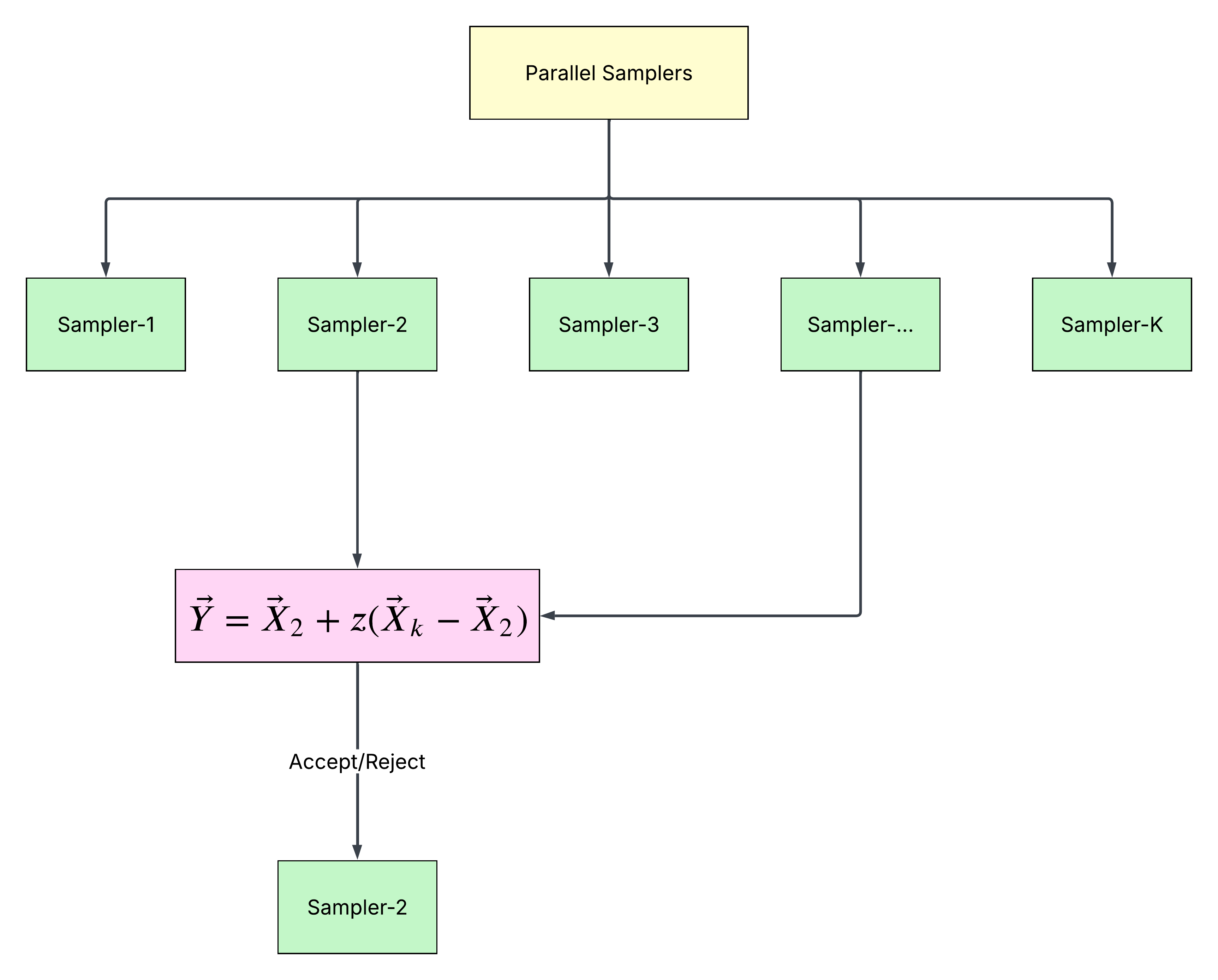
where \(z\) is drawn from,

\[g(z) \propto \frac{1}{z},\ \ \ \ \ z \in [\frac{1}{a}, a]\]

with \(a = 2\) by default.

For the DREAM method, an illustrative diagram is presented below,

DREAM

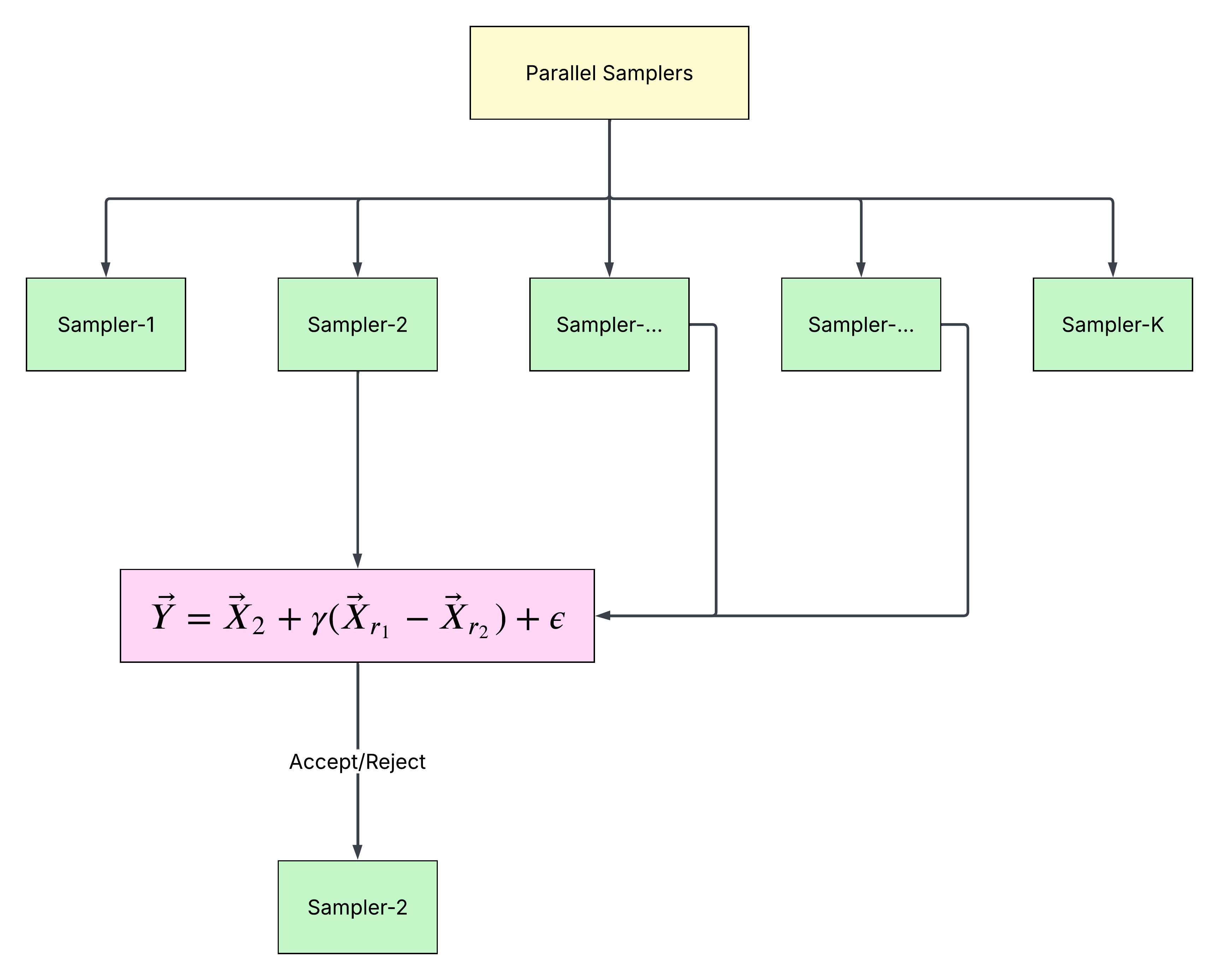
which takes a similar idea as with the Emcee method to run multiple samplers simultanesouly and uses the parameter difference between samplers to update the current sampler. With Emcee, the difference is between the current sampler and another randomly picked sampler. For DREAM, the difference is between two randomly picked samplers other than the current one. With DREAM, there are also some tunable parameters like the jump factor \(\gamma\) and the noise term as shown in the formulation in the diagram. Also, during the DREAM optimization, there is a stage called burn-in where the sampling is only for pinning down some hyperparameters for controlling the sampling and therefore all samples in the burn-in stage will be forgotten. Typically, we need to determine the crossover menu (a list of probabilities) to control the random picking of a certain proportion of parameters (say, \(1/2\), \(1/3\) or \(1\)) to sample at each stage (changes for all parameters not picked will be forced to 0). More detailed explanation about both algorithms is beyond my current capacity and understanding. Maybe at some point in the future I will come back to the topic again. We will see. For the moment, I redirect the further reading to Refs. [8, 9].