With a collection of data, we may want to extract or estimate the underlying distribution model. For example, we have the collection of house price in a certain area, we want to have an idea about how the house price in that area is distributed. However, without a priori knowledge about what the model that distribution should follow, we cannot follow the so-called parameterized way for estimating the distribution. In that way, we know beforehand about what the distribution model should be and it’s just some parameters yet need to be determined. Then we can do the commonly used least-square fitting to obtain those unknown parameters. However, it is usually the case where we have no knowledge about what the distribution model should look like, in which case we need a non-parameterized approach to estimate the underlying distribution, e.g. the histogram method and the one we are going to focus here: kernel density estimation (KDE).
Here is the formulation of KDE,
where \(h\) is called the bandwidth which plays an important role in determining our estimation for the distribution density. \(K\) is just our kernel function, for which we may have several alternative choices - a Gaussian kernel is usually used. Detailed introduction about mathematics of KDE can be found in Ref. [1] and we are not going to reproduce them here. Instead I put several key points as follows, which I think is quite important for better understanding the KDE method,
- Wherever we have an observed data, we should put a corresponding kernel there.
- The kernel function we put at each observed data point is a normalized distribution function, for which the probability density is the highest at each corresponding observed data point.
- The fundamental idea behind the kernel approach is that around each observed data point, the further we go away from the observed data point, the less our probability density should be.
- The overall sum of all the kernels should be normalized to 1, i.e. the overall probability should obviously be 1.
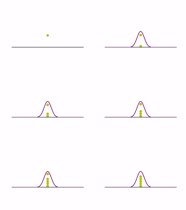
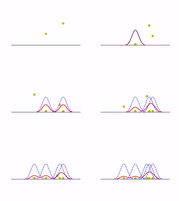
There are more technical details about KDE, for which one can refer to the introduction given by Ref. [1]. Here we use two simple animations to demonstrate the idea about KDE, as presented below,


The left-hand side figure gives the situation where all five data points fall onto the same position and the KDE distribution stays all the same as we have more data coming. The right-hand side figure gives more general situation where all five data points fall onto different positions, from which one can clearly see how the estimation of KDE distribution varies as we collect more and more data points.
========================I AM A SEPARATOR========================
☝About the influence of norm choice upon KDE for higher dimension
The idea of KDE can be easily extended to higher dimensions and the idea is still the same - the further we go away from the center of a specific kernel, the less distribution probability we will have. However, for high dimensions, it is not as straightforward as it is for 1D case, in terms of how we define the distance from the kernel center. Mathematically, the distance we mean here is actually a norm of a certain type, e.g. L0 norm, L1 norm or L2 norm, … According to the definition of norm,
\[||\vec{x}||_p = \sqrt[\leftroot{-1}\uproot{5}p]{\sum_i |x_i|^p}\]
where \(p\in{\rm I\!R}\). For 1D situation, the value of various different L norms is the same (except L0 norm, which is kind of special - see note below), since simply we have only one entry in the vector. But going to higher dimensions, we have more entries in the vector and therefore different L norms do give different distances. Therefore, choosing different L norms for the KDE analysis will influence the results, especially when we have limited number of input data points. Detailed discussion about the influence of different L norm choices can be found in Ref. [1].
N.B. There are two special L norms - L0 norm and L-Infinity norm - among which L0 norm is even more problematic since we don’t have rigorous definition for what \(\sqrt[0]{n}\), where \(n\neq 0\). Therefore, in practice, the L0 norm is actually defined as,
where \(\#\) means ‘the number of’. As for the L-Infinity norm, it means the maximum entry in the vector component. This is relatively straightforward to follow - given the mathematical definition of L norm above, the maximum entry will be the only one dominating as compared to all the other entries, considering the infinity power.
Refer to Ref. [2, 3] for more detailed discussion about L norms.
References
[1] https://www.youtube.com/watch?v=x5zLaWT5KPs&list=PLAYk0l7EXZVumN_Uil7ou8WUBkrFkVE91
[2] https://rorasa.wordpress.com/2012/05/13/l0-norm-l1-norm-l2-norm-l-infinity-norm/
[4] https://www.evernote.com/l/AQpVf7ClpwZJp7qhPTXWRPHUZL2MAIUC40E