Image generated with Gemini with the prompt ‘generate an image for me as an interesting head image in my Bayesian optimization post. when people see the image, they know the post is talking about the BO. but it should not be an illustrative image showing details of BO. just an abstract one should be fine. use the Ghibli art style’.

Background – Gaussian Process

In practice when we are dealing with optimization problems while the parameter space is huge to explore, we need some methods to guide us to explore the parameter space in an efficient way. For example, when synthesizing multi-component high entropy alloy (HEA) materials, if we want to tune the composition to target at optimal hardness or whatever material properties, the exploration space is exploding. The brutal force way of trying out composition combinations is inefficient until it becomes practically impossible due to high dimensionality of the configuration space. Suppose we have a model and if we feed in the coordination in the configuration space (e.g., a specific combination of composition) into the model and the model will spit out the property, that will be perfect since we know exactly where to go in the configuration space for the exploration. For sure, if we do have such a model, then we don’t need to explore at all since we know exactly where to go to target at the property with the exact model. Well, the thing is, in practice, we never have such a model, I mean the exact deterministic model. But indeed we can have some model, some probabilistic model, to help us. Gaussian process is one of such models – based on those measured points (e.g., a certain set of synthesized HEA samples with specific compositions, together with the corresponding measured properties) and a simple principle that the closer that points in the high dimensional space are getting to each other, the closer that their corresponding values should get to each other, the mean value and the variance of unknown points in the configuration space can be predicted.

I have some detailed summary slides about Gaussian process in Ref. [1] and I won’t reproduce all the details here but instead I will just put down the main results. Say the high dimensional configuration space is represented by \(\mathbf{X}\) and we have data \(Y = m_1\) at \(\mathbf{X} = \mathbf{x}_1 = (x_1=0.5, x_2 = 0.1, x_3 = 1, x_4 = 5, \dots)\), \(Y = m_2\) at \(\mathbf{X} = \mathbf{x}_2 = (x_1 = 1, x_2 = 0.7, x_3 = 2, x_4 = 0.8, \dots)\), etc. Based on the available data, we want to predict at \(\mathbf{X} = x_*\). Putting \(\mathbf{x}_1\), \(\mathbf{x}_2\), \(\dots\) and \(\mathbf{x}_*\) altogether, their values follow the joint Gaussian distribution,

Here, \(f_*\) refers to the value at \(\mathbf{X} = \mathbf{x}_*\) that we want to predict. For points without data, we can have some prior function \(m(\mathbf{X})\), the choice of which is up to us. For example, we can just choose to have \(m\mathbf{X} = 0\). In the joint Gaussian distribution formulation above, \(m_* = m(\mathbf{X} = \mathbf{x}_*)\). Now comes the covariance matrix part. To specify all the terms in the matrix, we need to first give a kernel function, which is a function up to our choice and defines how different points in the configuration space are correlated to each other. Basically, all the terms in the covariance matrix for the joint Gaussian distribution are constructed from the kernel function and we know that the covariance matrix defines the correlation between the distribution of various variables, or, in the context of current post, the correlation of values for different points in the high dimensional configuration space. So, even without writing down the specific form of the matrix components, we know that the kernel function definitely is something to do with the correlation. Specifically,

Putting all together,

Here, terms like \(k(\mathbf{x}_1, \mathbf{x}_1)\), \(k(\mathbf{x}_1, \mathbf{x}_2)\), etc. are evaluated by putting the coordinates in the high dimensional space into the kernel function we picked. For example, if we choose to use the Radial Basis Function (RBF) kernel, the function is,

where \(\ell\) and \(\sigma_f\) are both hyperparameters.

Finally, to give the estimation at \(\mathbf{x}_*\), we need to calculate the conditional distribution, i.e., the distribution of the single variable \(f_*\) with all the other values at all the observed points are fixed,

Now, given all the already observed/measured data, we can predict the mean and variance for any points in the configuraiton space. This is critical for us to make decisions about what is next. In the machine learning terminology, determining ‘what is next’ can be treated as ‘to pick a new training data’ – indeed, it is. Like with the Gaussian process, we have some observed data and we use them to construct a model to predict values and variance at an arbitrary point in the configuration space. Then if we somehow utilize such information to pick a new point to observe or take the measurement at, we are indeed adding a new data point to the training data so that when predicting the next one, the data added in the current step will be incorporated into the model construction. In general, such a process of adding new training data into the learning process on-the-fly, in machine learning, is called active learning.

Bayesian Optimization

Having established the formulation for Gaussian process, we are ready to discuss how we can use it for making decision about what is coming next. One thing we can do is obviously to directly use the information coming out from the Gaussian process. Across the whole configuration space \(\mathbf{X}\), the Gaussian process gives us the estimation for the mean and variance for the value at each point. So, an obvious step to take is to take a measurement at those points with large variance (i.e., with large uncertainty) – this is considered as being exploration since the sampling happens where the model is most uncertain. However, with such an approach (i.e., being purely exploratory), the mean information obtained from the Gaussian process is unused at all. Suppose we are trying to optimize something, e.g., the hardness of HEA by tuning the composition, not only we want to explore those configuration points where the model is uncertain, but also we want to seriously consider the points where the model thinks the hardness is maximized. Then, we step into the Bayesian Optimization (BO).

BO is about balancing the utilization of both pieces of information – the mean and variance that we obtained from the Gaussian process. There are three main approaches in impelmenting the BO,

• Lower/Upper Confidence Bound (LCB/UCB)

• Probability of Improvement (PI)

• Expected Improvement (EI)

Let’s discuss them one by one and we will see how the BO is realized in practice.

Lower/Upper Confidence Bound (LCB/UCB)

First, the LCB/UCB.

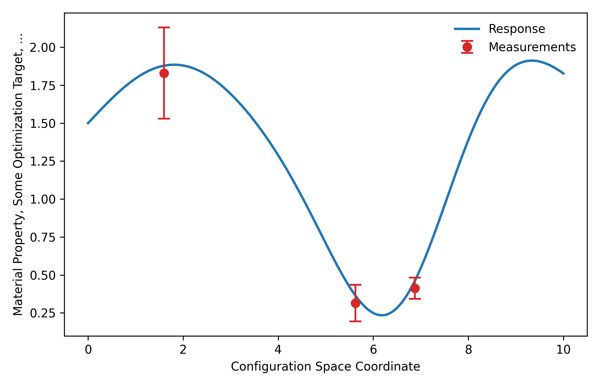
In the case shown above, let’s say we have the Gaussian process predict the mean and variance for several points (red points) – the blue curve is the underlying ground truth. If we were to decide which point to go next for taking the observation based on the prediction, the pure reliance on the variance tells us to go with the point on the very left. However, if our target here is to find the minimum of the curve, ignorance of the predicted mean values is obviously not an optimal thing to do here. Though, we don’t want to purely rely on the predicted mean values either and therefore instead we look at the following quantity,

where \(\kappa\) is a pre-chosen hyperparameter (e.g., \(\kappa = 2\)). Since the value at each point is assumed to follow the Gaussian distribution, for a given value of \(\kappa\), the following probability is the same for all points,

Another way to look at this is to define a variable \(U\) as,

Referring to the Gaussian distribution formulation, we know that \(U \sim \mathcal{N}(0, 1)\) since \(m(\mathbf{x}) \sim \mathcal{N}[\mu(\mathbf{x}), \sigma(\mathbf{x})]\). So the probability above becomes,

where \(\Phi\) is just the Cumulative Distribution Function (CDF) corresponding to the Gaussian distribution \(\mathcal{N}(0, 1)\). If we set \(\kappa = 2\), we have \(\Phi(-2) \approx 0.02275\), which can be regarded as a small number, meaning that the probability of \(U\) being smaller than \(-\kappa = -2\) is very small. This is to say that the probability of \(m(\mathbf{x})\) being smaller than \(\mu(\mathbf{x}) - 2\sigma(\mathbf{x})\) is very small. So, the value \(\mu(\mathbf{x}) - 2\sigma(\mathbf{x})\) sets the Lower Confidence Bound (LCB) for our prediction. What does this mean? Say we have a large value of LCB at a certain point (e.g., the point on the very left side in the figure above), the LCB tells us that there is little chance for \(m(\mathbf{x})\) to be smaller than the LCB. So if the LCB value is large, that means we have a very little chance to get a small value than the LCB. If we are trying to find the minimum, points with large LCB are definitely not what we want. Then our sampling condition become clear – we just need to take the Gaussian process predictions at all grid points in the configuration space and find out the one with the smallest LCB and that point will be our next observation point.

Probability of Improvement (PI)

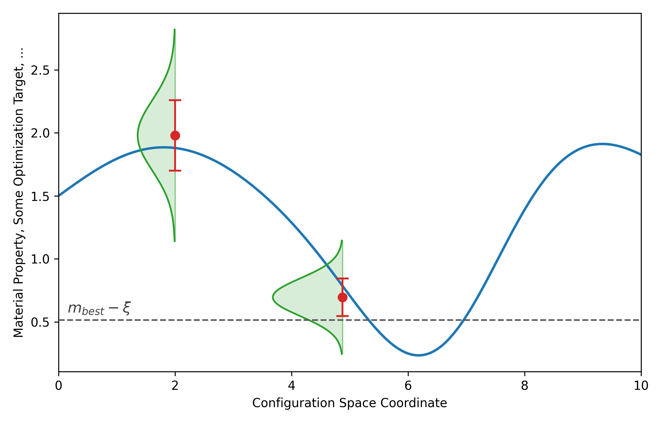
Suppose at the current step of the optimization, we have the minimum value as \(m_{\text{best}}\). Given a pre-chosen margin \(\xi\) (which can be tuned as a hyperparameter), we want to ask such a question – at a certain configuration point \(\mathbf{x}\), what the probability is for \(m(\mathbf{x})\) to be smaller than \(m_{\text{best}} - \xi\), i.e.,

Notes about the margin \(\xi\)

By introducing the margin \(\xi\), we are not only interested in the new sampling is getting better than the current optimum, but also interested in getting much (inferred by the pre-defined margin \(\xi\)) better.

Again, we define \(U\) in the same way above,

and effectively we are looking at the probability,

Defining,

we have,

which is the quantity we want to maximize regarding the decision to make about what is to sample next. Taking the example presented in the figure above, we see that for the candidate point on the left, the value of \(\text{PI}(\mathbf{x}_{\text{left}})\) should be very small. As for the point on the right, the area under the green Gaussian distribution probability density functio (PDF, and below the dashed line indicating the \(m_{\text{best}} - \xi\) level) should yield a much larger value. If we were to pick between the two points to try next, with the PI approach, we will for sure change the point on the right.

Expected Improvement (EI)

There are some obvious issues with the PI approach. First, let’s say we have two points in the configuration space, as below,

• Point A: \(\mu_A = m_{\text{best}} - 1\), \(\sigma_A = 1\)

• Point B: \(\mu_B = m_{\text{best}} - 10\), \(\sigma_A = 10\)

For the demo purpose, let’s just choose the margin \(\xi = 0\) and we will see the value of \(z\) for both of the two points is \(z = 1\). Therefore,

So, the PI approach gives identical outcome for both points and does not give useful advice on which one to sample next. However, we know that between the two points, we do want to sample point B since it has high uncertainty (therefore worth exploring). The PI approach hits the failing spot in this imaged situation. From the example here, we can see that the fundamental reason for the failure of the PI approach is that the uncertainty comes into the PI evaluation only in the form of a division factor and therefore it will normalize out the actual difference between the prediction and the current optimum.

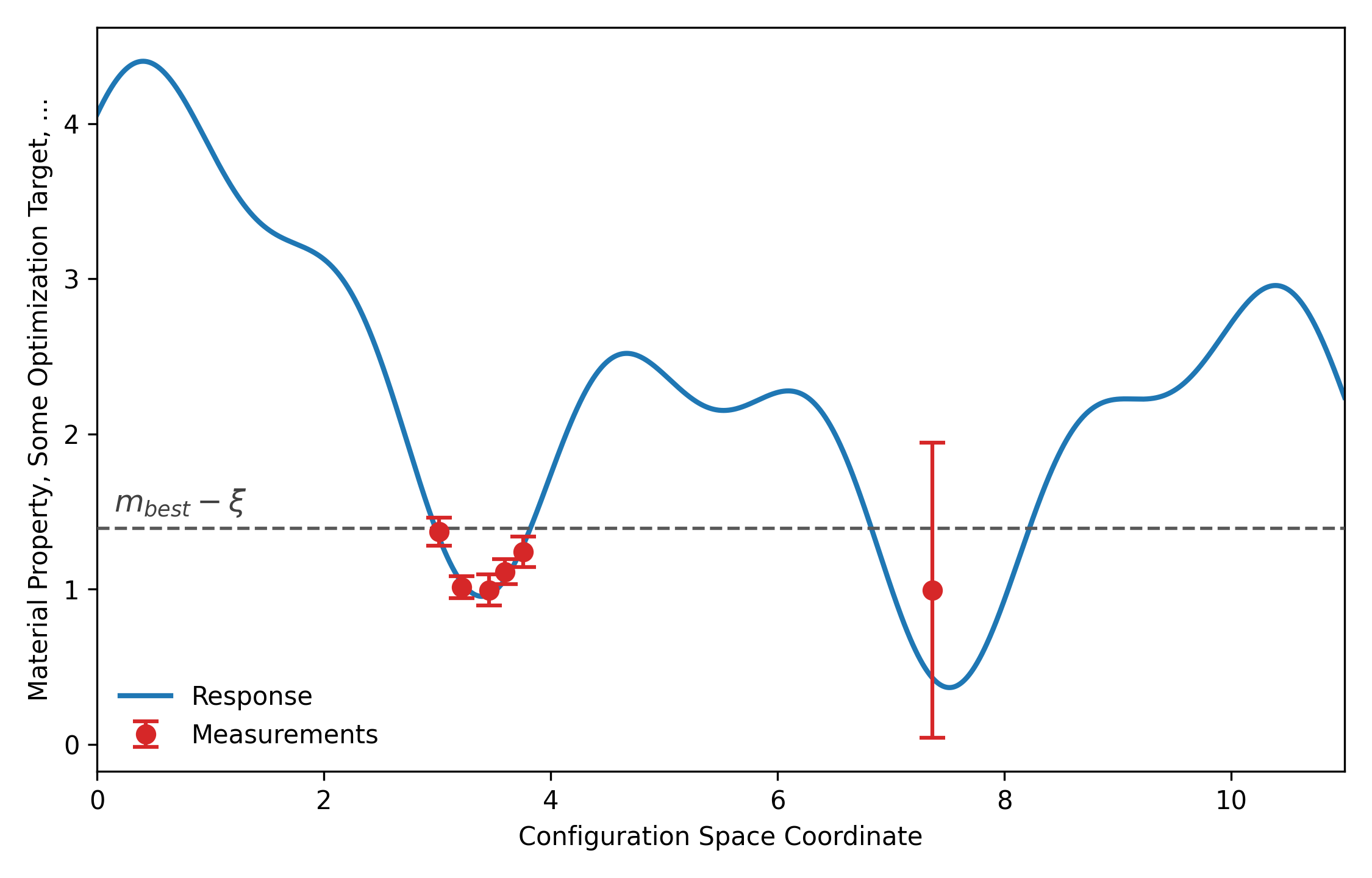
Another failing spot of the PI approach is shown in the figure above – in this case, it is about the over-exploitation, i.e., the loss of exploration. Among all the candidate points to try out next, all those points on the left side near the local minimum are with obviously larger \(z\) values as compared to the single point on the right side. This is mainly because the variance of the point on the right side is predicted to be large. So, all the points on the left are considered reasonable next sampling points – the BO process in this case tend to wander around the local minimum without strong ‘willingness’ to explore other regions.

The EI approach can hopefully help in such cases. The Expected Improvement, as suggested by its name, calculates the expectation,

where,

The formulation needs a bit explanation. First, still we have the quantity \(m_{\text{best}} - \xi\) indicating the currently identified optimal (e.g., the minimal) value minus some pre-defined margin \(\xi\). With the margin term, nothing fundamentally is changed – it is just that we are more aggressive in terms of getting better. \(\text{max}(m_{\text{best}} - \xi - m, 0)\) says, if the prediction is getting worse, i.e., \(m\) is larger than the current optimal value by the pre-defined margin, we will cap the value at 0. When it is getting worse, we are not at all interested in by how much it is getting worse – the whole worse part in the predicted distribution therefore contributes \(0\) to the expectation value evaluation. Given in its integration form, we have,

where \(\text{max}(\cdot, 0)\) kills the integrand wherever \(m > m_{\text{best}} - \xi\). Also,

where \(\phi\) is the standard normal PDF,

and here I am writing \(\mu = \mu(\mathbf{x})\) and \(\sigma = \sigma(\mathbf{x})\) for brevity. Here, let’s just substitute,

so,

and the integration upper limitation just transforms as,

where we replace \(m\) with \(m_{\text{best}} - \xi\) in the defined variable \(u\) above. The integral therefore becomes,

where \(\Phi(z)\) is just the CDF for the standard normal distribution,

For the second term in the integral, we have,

so, the integrand in the second term becomes,

and therefore,

Putting together both terms, we have the EI value given as,

where we see that the uncertain \(\sigma\) appears as a prefactor of an additive term – not like in the PI approach where it appears only in the normalization term. Therefore, we will not have the normalization issue as mentioned above for the PI approach. Meanwhile, the additive term containing the uncertain yields a better balancing between the exploitation and exploration. In practice, with the EI approach, we decide the next sampling step according to,

Notes about the maximization problem

Here in the post, I am mainly focusing on the minimization problem with BO. In practice, maximization is another typical type of optimization task. There is really not that much extra to say about maximization beyond the formulation and explanation in the post. Simply negating the quantity to maximize, the maximization problem will be easily turned into a minimization problem.

Pros & Cons for the Three Measures

LCB/UCB

Pros: Highly intuitive – for the example, the LCB \(\mu(\mathbf{x}) - \kappa\sigma(\mathbf{x})\) explicitly balances between exploitation and exploration. Also, the \(\kappa\) hyperparameter can be adjusted on-the-fly so that we have the direct control over the trade-off during the BO process.

Cons: Relies strongly on the choice of the hyperparameter \(\kappa\).

PI

Pros: A good choice if the main goal is improvement regardless of size, or when the potential risk is expensive to take.

Cons: Highly explotative. Easy to be trapped in local optima.

EI

Pros: A robust “default” choice, with better balancing between exploitation and exploration.

Cons: Mathematically a bit more complex to evaluate but should not be a big deal in practice.

Some Useful Resources

• A cookbook going over Bayesian optimiztion and active learning can be found in Ref. [2].

References

[1] https://www.overleaf.com/read/kzhbrfhkfsng#77c4d9

[2] https://www.physicsx.ai/newsroom/bayesian-optimization-and-active-learning-cookbook