Introduction
In this post, I am going to put down some notes on a very nice paper by Prof. Z. T. Chen from UT Austin. The paper implements a physics model guided Bayesian optimization for spectroscopy experiment steering [1]. As a high-level summary, the backbone of the paper is as below,
-
A certain sample orientation corresponds to a specific set of \(S(\mathbf{Q}, E)\) map.
-
To guide the experiment (before which, for sure, we don’t have any data), we need to calculate the \(S(\mathbf{Q}, E)\) map somehow.
-
Calculation of the \(S(\mathbf{Q}, E)\) map can take two routes,
-
Use physics models, relying on the given Hamiltonian to use dynamis calculation packages for the calculation \(\Rightarrow\) practically unfeasible since the downstream tasks (typically, the utility function and likelihood evaluation to be mentioned below) requires heavy computation efforts over many grid points (e.g., the coupling parameters and sample orientation).
-
Surrogate model \(\Rightarrow\) practically feasible and requires dedicated machine learning model training.
-
-
With either route, the \(S(\mathbf{Q}, E)\) map calculation relies on the coupling coefficients. So generally, we have \(\hat{S}(\mathbf{Q}, E \vert \vec{\theta}, \xi)\), where \(\vec{\theta}\) refers to the coupling coefficient with multiple components (e.g., \(J_1\), \(J_2\), etc.) and \(\xi\) refers to the sample orientation.
-
Here, \(\vec{\theta}\), \(\xi\) and \(S(\mathbf{Q}, E \vert \vec{\theta}, \xi)\) can all be generalized. \(\xi\) is something like sample or experiment configuration that we may want to steer during the experiment. \(S(\cdot\vert \vec{\theta}, \xi)\) is the modeling for the physical quantities we will be measuring and \(\vec{\theta}\) is the parameter that controls the modeling.
-
The fundamental problem that the paper solves is like this – we want to use the modeling for the physical quantities to guide our sampling for the sample or experiment configuration. Sure, no problem. However, the modeling requires a good knowledge about \(\vec{\theta}\), and without the full volume of measurement data, there is no reliable way to obtain \(\vec{\theta}\). This puts us in a dilemma. The way out is, we have some prior belief for the \(\vec{\theta}\) distribution and we keep updating the posterior distribution given the continously measured new data on-the-fly, based on the Bayesian rule. This is the
physicspart of the reported framework. As for thesteeringbit of the framework, based on the posterior \(\vec{\theta}\) distribution, somehow we can figure out a utility function (see details below) to help us make the decision on the next sampling point (represented by \(\xi\)).
Evaluation of the Expected Information Gain (EIG)
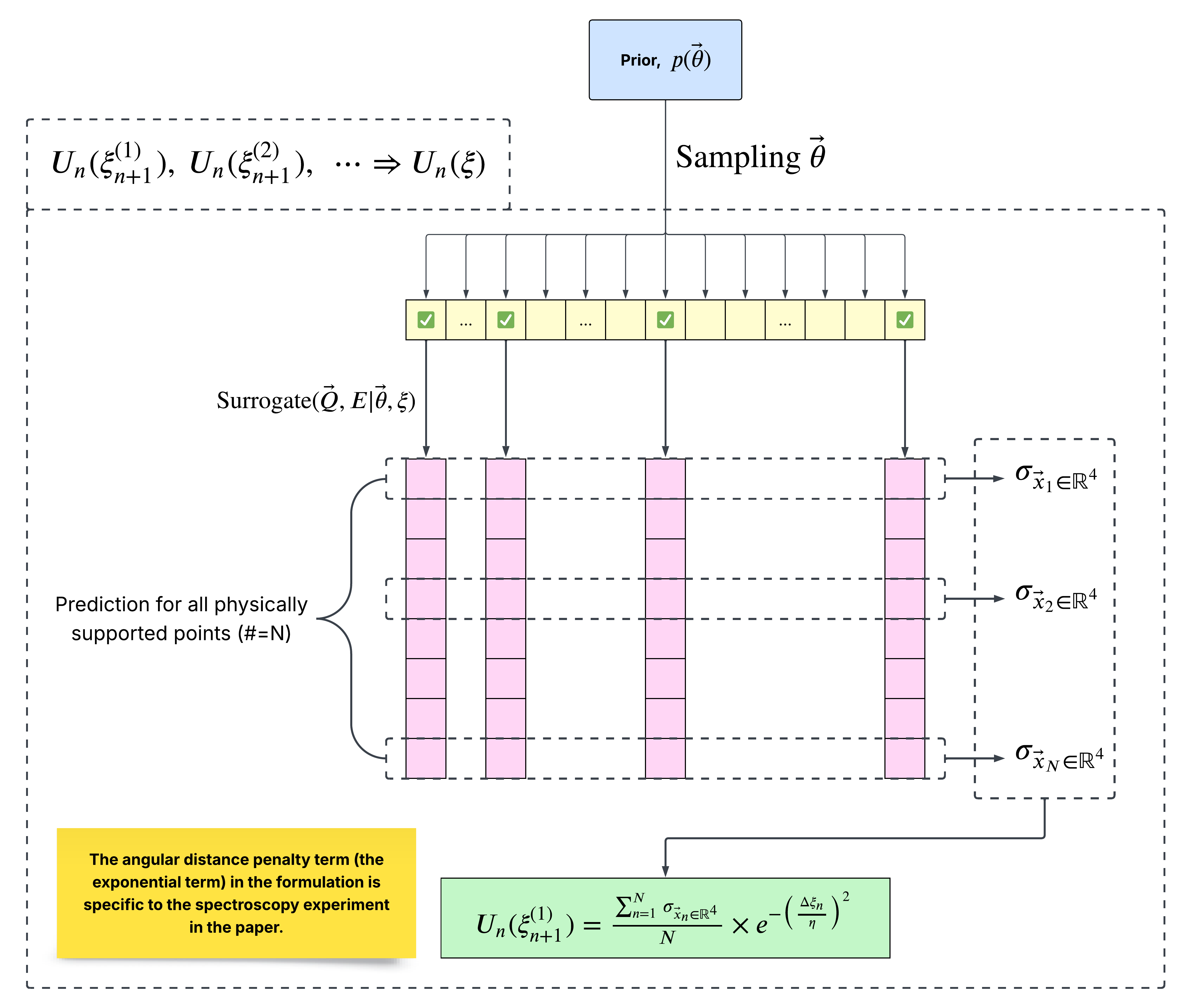
Here is presented the summary of the algorithm for evaluating the Expected Information Gain (EIG),
Right click on the image and select
Open image in a new tab(or something similar) to view a larger version of the image.
Some notes on the workflow,
-
The prior distribution \(p(\vec{\theta})\) is not analytical but instead it is just probability values attached to the discrete \(\vec{\theta}\) grid.
-
After the update with the new observed data, the posterior will be come the new prior, therefore forming an update loop.
-
For the evaluation of the utility function, only a portion of the sampled \(\vec{\theta}\) is used.
-
Along the vertical direction, each of the pink boxes represents a single observable coordinate in the 4D space (\(\vec{Q} \Rightarrow 3, E \Rightarrow 1\)). For each of the coordinate, we have the predicted value corresponding to each of the \(\vec{\theta}\) from which we can calculate the standard deviation, as shown in the figure.
-
The utility function presented here is what the paper finally takes but it is only an approximate form of the full version. The paper presents the full version and some notes generated by Claude can be found here.
$U_n$ is the utility function (the Expected-Information-Gain-style acquisition function) evaluated using everything known up through step $n$ – i.e., using the current posterior over $\vec\theta$ (drawn as the “Prior, $p(\vec\theta)$” box and sampled in the diagram). So,
\[U_n(\xi_{n+1}^{(1)}),\ U_n(\xi_{n+1}^{(2)}),\ \dots \ \Rightarrow\ U_n(\xi)\]means: score each candidate configuration one at a time, and stitching all those scores together across the whole candidate grid gives you the full utility function $U_n(\xi)$, which you then maximize to pick the actual next measurement point.
Likelihood
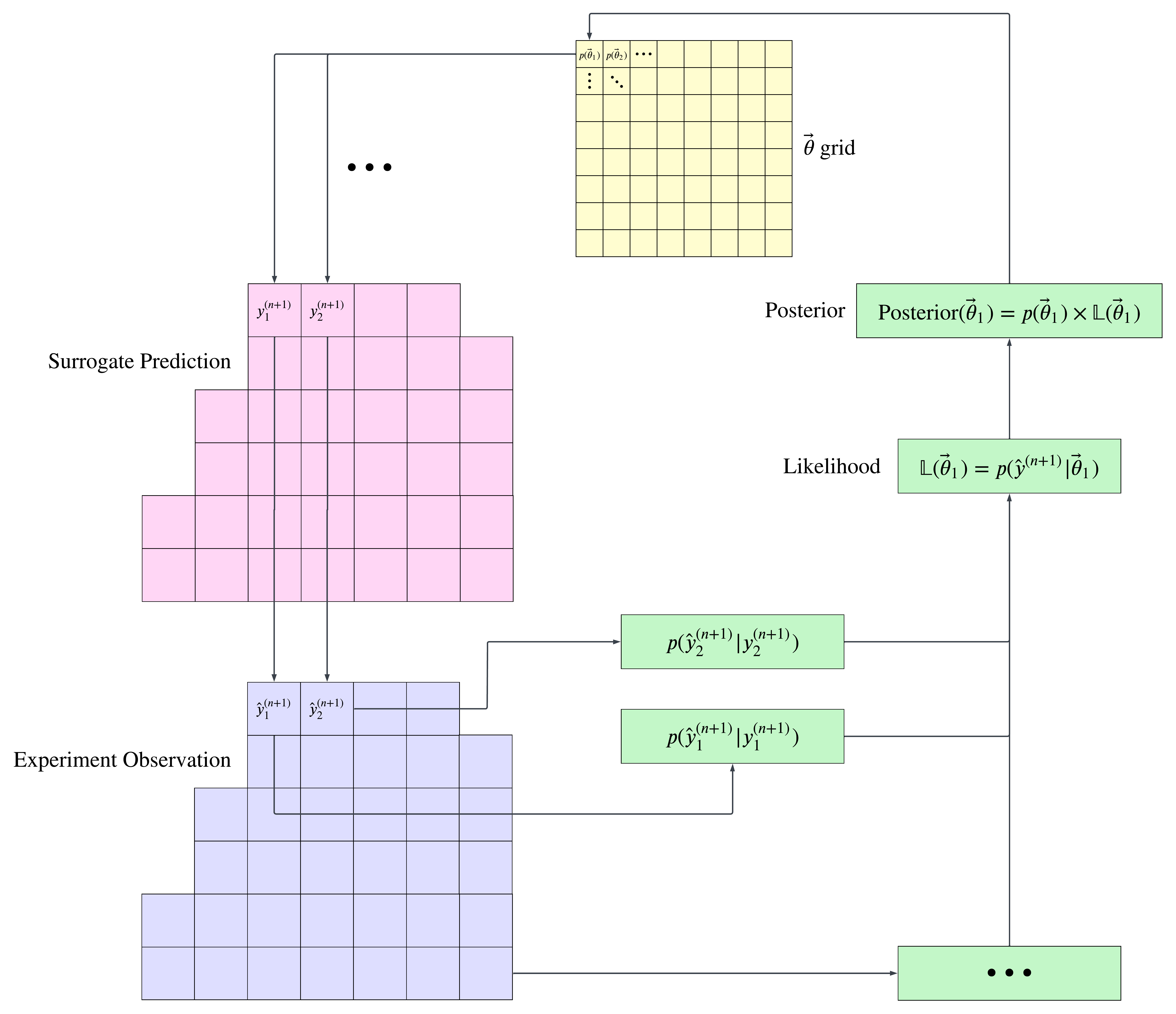
Here is presented the summary of the algorithm for evaluating the likelihood,
Right click on the image and select
Open image in a new tab(or something similar) to view a larger version of the image.
Some notes on the workflow,
-
The evaluation of the overall likelihood for a given \(\vec{\theta}\) (\(\vec{\theta}_1\), \(\vec{\theta}_2\), etc.) requires the evaluation of the likelihood of observing the actually observed intensity \(\hat{y}\) for a single coordinate in the 4D space (represented by pink squares in the figure) in the \((n + 1)^{\text{th}}\) step (i.e., the just measured step).
-
We need to run the loop presented in the figure for all the \(\vec{\theta}\) values and for each \(\vec{\theta}\), the exactly computed values \(y_1^{(n + 1)}\), \(y_2^{(n + 1)}\), etc. can be obtained. Then assuming the Poisson noise, the probability of actually observing the observed intensities \(\hat{y}_1^{(n + 1)}\), \(\hat{y}_2^{(n + 1)}\), etc. can be calculated, individually. Here the exactly computed values \(y_1^{(n + 1)}\), \(y_2^{(n + 1)}\), etc. incorporates the instrument resolution effect – refer to the details presented in the paper.
-
All the likelihood values for each individual 4D coordinate need to combined together to give the likelihood that will be used for calculating the posterior. Here two things to note, 1) only a portion of the 4D coordinates are picked for the calculation for the computational consideration and 2) the individual likelihood values are just averaged to give the likelihood that is not a rigorous representation of the actual likelihood (see the paper for justification of doing so).
-
As shown in the figure, for each of the \(\vec{\theta}\) values, the finally obtained posterior will be used as the prior for the next overall loop.
-
The figure presented here is actually just the overall loop – the utility workflow presented in the previous figure should sit on the arrow pointing from the pink squares to the light magenta squaures, i.e., it is used for determining where to measure \(\hat{y}^{(n + 1)}\).