
Image generated with Gemini with the prompt ‘generate an abstract image for demo of Poisson distribution pictorially. use the Ghibli style’.
Introduction
Poisson distribution is usually used to describe the distribution of independent discrete events happening in a constant rate. For example, in neutron scattering experiments, detectors record the events of neutrons hitting the detector. Such events can be described by the Poisson distribution, because,
-
The number of neutrons hitting the detector is discrete, i.e., we cannot have 0.5 neutron recorded to hit a detector.
-
Normally the event of each individual neutron hitting a detector is independent from each other.
-
For a certain detector or a specific point in the measurement space (e.g., \(Q\) for powder diffraction, \((\vec{Q}, E)\) for spectroscopy), the number of neutrons being recorded per unit time is considered as a constant, for a specific measurement.
Mathematically, the Poisson distribution describes the probability of observing a certain number of events in a certain time interval, given the average observation rate. For example, if the number of neutrons corresponding to a certain \(Q\) point (i.e., \(Q \rightarrow Q + d\,Q\)) in a powder diffraction measurement is \(10^7\) per second, the actually observed number of neutrons follow the Poisson distribution with the constant rate of \(\lambda = 10^7\).
Given a structure model of the measured sample, the scattering intensity at \(Q\) points can be calculated to an absolute scale, given in the unit of cross section. Knowing the incident neutron flux, the number of scattered neutrons for \(Q\) points can be calculated, which will be our average counting rate.
The probability mass function (PMF) for the Poisson distribution is,
\[P(N) = \frac{(\lambda t)^N e^{-\lambda t}}{N!}\]Here, \(t\) here is the time interval that can be specified by us to indicate the duration of interest, e.g., we can set it to \(1\) for the unit time interval. \(\lambda\) is the constant rate as mentioned, indicating the average number of events in one unit time, e.g., the average number of neutrons per second.
For discrete distribution, the probability mass function is used to give the probability for each observable outcome.
Characteristic quantities
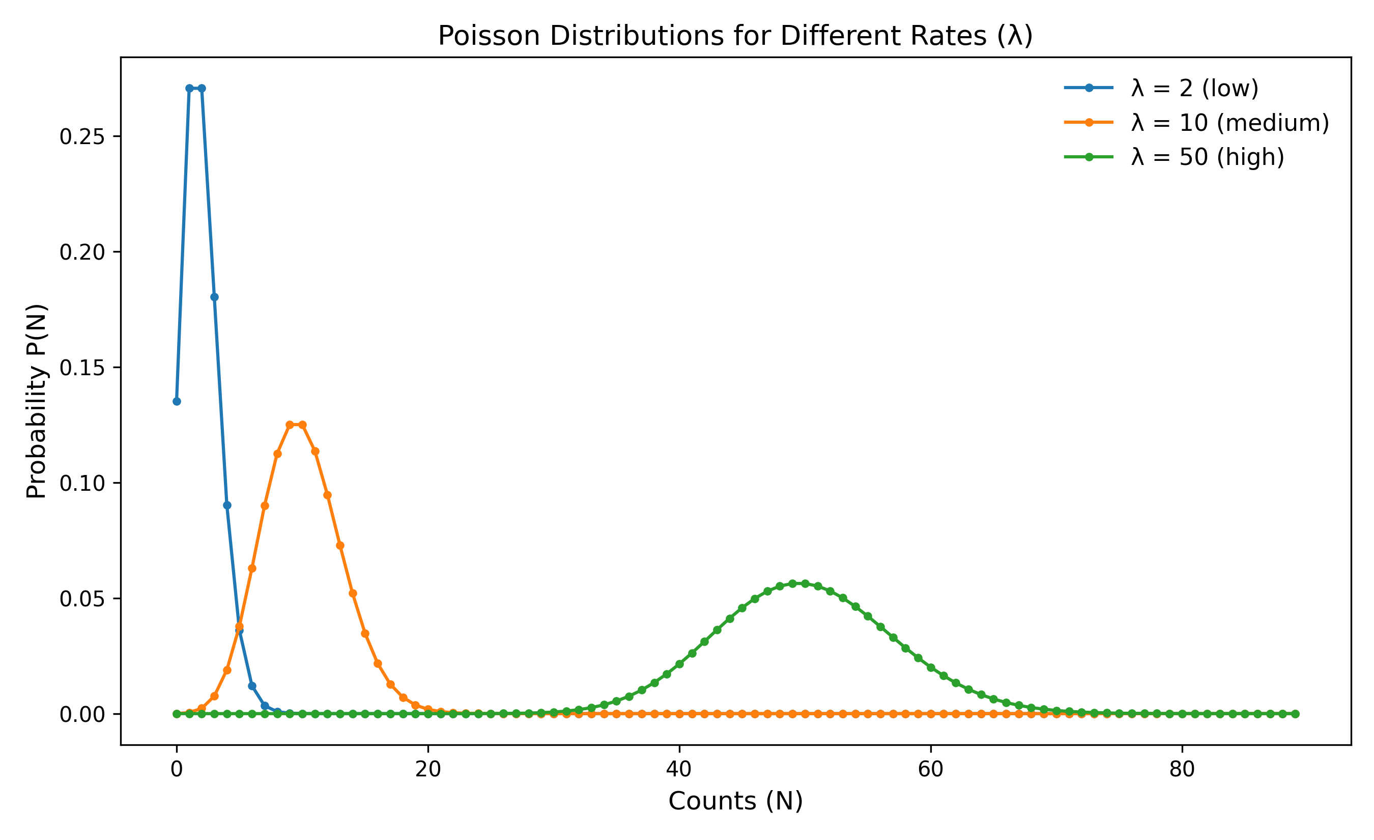
The figure here shows the PPMF for several different Poisson distributions with different constant rate. Visually, the characteristics look very much different, and in practice, we have quite a few quantities for general probability distribution to describe their characteristics. Some obvious quantities that would immediately pop up in our minds include the mean and variance, and there are more than that – refer to the Related terms session in Ref. [1] for a list of such quantities. Here I am only noting down several of the quantities,
-
mean,medianandmode: These quantities all give us some idea about the typical value of the random variable. When dealing with a general random distribution, there is no golden choice of those quantities as the representative of the random varable value. Instead, it is just a matter of choice.modeis probably the most straightforward one (at least visually) – it is just the value corresponding to the highest point in the probability distribution function (PDF) or the PMF.medianmeans such a value that half of variable values are above the value and half are below. For PMF, it is simply the number counting – we draw a vertical line on the PMF plot, count the number of points located to the left and right of the line no matter how far those points extend to, and as long as the numbers for left and right are equal, that line is ourmedian. For PDF, themedianis the line for which the area below the PDF on the left and right is equal.meanis the weighted average of the random variable – we multiply the variable value with its corresponding probability and sum them all up, and for PDF, this becomes an integration. Withmean, we are calculating thecenter of mass– if thinking of the random variable value as the weight, then if we separate the distribution by themeanline and put the left and right part on either side of a balance, the balance will, well…, balance.For a symmetric distribution, like the Gaussian distribution, the three quantities agree with each other. For asymmetric distributions, like the Poisson distribution, they usually do not.
-
\[\text{Kurtosis} = \frac{E[(X - \mu)^4]}{\sigma^4}\]kurtosis: This is a quantity that characterizes how significantly the tail matters, which helps answer such a question ‘do we expect a lot of outliers?’. The definition of kurtosis is,Usually, we also define the
\[\text{Excess Kurtosis} = \frac{E[(X - \mu)^4]}{\sigma^4} - 3\]excess kurtosisto use the kurtosis of the Gaussian distribution as the baseline,Three regimes:
-
Excess kurtosis = 0 (mesokurtic): normal-like tails.
-
Excess kurtosis > 0 (leptokurtic): heavier tails and a sharper peak than a Gaussian. More probability mass sits in extreme outliers.
-
Excess kurtosis < 0 (platykurtic): lighter tails, flatter/more spread-out peak. Fewer extreme outliers than Gaussian.
In the figure presented above, we see that the distribution of the random variable gets more spread-out as we have larger \(\lambda\), and therefore visually it seems flatter. Accordingly, more probability mass sits near the peak area so that we are expecting less outliers. Indeed, the kurtosis for the Poisson distribution gets smaller as the \(\lambda\) increases – excess kurtosis for the Poisson distribution = \(1/\lambda\).
-
-
\[\text{skewness} = \frac{E[(X - \mu)^3]}{\sigma^3}\]skewness: This is a quantity describing the asymmetry of the distribution, defined as,Since the exponent \(3\) in the top term is an odd number, the positive side (when the value of \(X\) ia greater than \(\mu\)) and the negative side (when the value of \(X\) ia less than \(\mu\)) contributes different sign (therefore asymmetrically). Hence it is understandable that the resulted quantity characterize the asymmetry of the distribution.
Rough rule for the evaluation of the asymmetry based on the value,
-
\(\vert \text{skewness} \vert < 0.5\): roughly symmetric
-
\(0.5\)-\(1\): moderately skewed
-
\(> 1\): significantly skewed
For the Poisson distribution, the skewness is given as \(1/\sqrt{\lambda}\).
-
-
\[\mu_n = E[(X - E[X])^n] = \int_{-\infty}^\infty (x - \mu)^nf(x)d\,x\]central moment: The \(n\)-th central moment about the mean \(\mu\) of a probability distribution is,where \(f(x)\) refers to the PDF of the probability distribution. As can be seen from the
kurtosisandskewnessdefinition above, both of them involve the central moment in the calculation.
Large \(\lambda\) reproduces the Gaussian distribution
As can be observed in the figure above, as the average constant rate of observation gets larger, the shape of the Poisson PMF gets closer to the shape of a Gaussian distribution. In this section, a detailed derivation will be presented. To fully lay out the proof, we need to put down some important notions involved in the proof.
Moment Generating Function (MGF)
For a random variable \(X\), the moment generating function is defined as,
\[M_X(t) = E[e^{tX}]\]Expanding \(e^{tX}\) as a power series,
\[e^{tX} = 1 + tX + \frac{t^2X^2}{2!} + \frac{t^3X^3}{3!} + \cdots + \frac{t^nX^n}{n!} + \cdots\]and taking expectations term by term (using linearity of expectation) gives:
\[M_X(t) = 1 + tE[X] + \frac{t^2E[X^2]}{2!} + \frac{t^3E[X^3]}{3!} + \cdots\]Comparing this with the general Taylor expansion of \(M_X(t)\) around \(t=0\),
\[M_X(t) = M_X(0) + M_X'(0)t + \frac{M_X''(0)}{2!}t^2 + \cdots\]shows that the \(n\)-th derivative of the MGF at \(t=0\) equals the \(n\)-th moment of \(X\):
\[M_X^{(n)}(0) = E[X^n]\]Thus, if the MGF is known as a function, all moments of the distribution can be recovered, and conversely, knowledge of all moments (as Taylor coefficients) can in principle reconstruct the MGF as a function – provided the underlying series converges to the true function, which is where analyticity becomes essential (discussed below).
Cumulant Generating Function (CGF)
The cumulant generating function is defined as the logarithm of the MGF,
\[K_X(t) = \log E[e^{tX}]\]Its Taylor coefficients at \(t=0\) are the cumulants \(\kappa_n\) of the distribution. The first few cumulants coincide with familiar quantities: \(\kappa_1\) is the mean, \(\kappa_2\) is the variance, and \(\kappa_3\) is the third central moment (used in skewness).
Analytic Functions
A function \(f(t)\) is said to be analytic at a point \(t_0\) if, in some neighborhood of \(t_0\), it is exactly equal to its own convergent Taylor series:
Analytic functions possess a rigidity property – two analytic functions that agree on all derivatives at a single point must agree everywhere on their shared domain of analyticity. This rigidity is what allows a full function to be reconstructed uniquely from a local sequence of derivatives (or moments).
For the argument to follow, it is essential that the MGF be analytic – not merely that its moments exist – so that knowledge of all moments genuinely pins down the entire function.
Characteristic Function
If the MGF \(M_X(t) = E[e^{tX}]\) is finite for real \(t\) in some interval \((-\delta, \delta)\), this finiteness extends naturally into the complex plane. Writing a complex argument as \(t = a + bi\),
\[e^{tX} = e^{aX}e^{ibX}\]Since \(e^{ibX}\) always has magnitude 1, the magnitude of \(e^{tX}\) depends only on the real part \(a\):
\[|e^{tX}| = e^{aX}\]Consequently, \(E[e^{tX}]\) converges whenever \(a \in (-\delta, \delta)\), regardless of the imaginary part \(b\). The set of such \(t\),
\[\{ t = a + bi : -\delta < a < \delta,\ b \in \mathbb{R} \}\]forms a vertical band in the complex plane – bounded in the real direction but unbounded in the imaginary direction – referred to as a strip. The imaginary axis (\(a=0\)) obviously lies within this strip since \(0 \in (-\delta,\delta)\). Because \(M_X(t)\) is analytic throughout this entire strip, it is fully determined by its Taylor coefficients (the moments) everywhere in the strip, it naturally follows that the analyticity at \(t=0\) is guaranteed. This infers the valid evaluation of \(M_X(t)\) at purely imaginary arguments \(t = is\),
\[M_X(is) = E[e^{isX}] = \phi_X(s)\]where \(\phi_X(s)\) is the characteristic function of \(X\). This equality holds for two distinct reasons. First, it is immediate from the definitions – substituting \(t=is\) into \(E[e^{tX}]\) produces exactly \(E[e^{isX}]\). Second, and more importantly, analyticity guarantees that this substitution yields a value consistent with the moment sequence – because \(M_X(is)\) equals the same Taylor series (now evaluated at an imaginary point) whose coefficients are the moments \(E[X^n]\). Without analyticity, one could only say the two sides happen to agree as expectations, not that the characteristic function is determined by the moments.
The characteristic function \(\phi_X(s)\) exists for every distribution. Further, a fundamental theorem – Lévy’s inversion (uniqueness) theorem – states that the characteristic function always uniquely determines the underlying distribution [2].
Taken together, these facts establish the chain: moments (near \(t=0\)) \(\rightarrow\) analytic MGF on a strip \(\rightarrow\) characteristic function via \(t=is\) \(\rightarrow\) unique distribution. This chain justifies working with cumulant generating functions to establish convergence in distribution, as carried out below for the Poisson case.
Poisson Approaches Gaussian as \(\lambda \rightarrow \infty\)
Let \(X \sim \text{Poisson}(\lambda)\), with mean \(\lambda\) and variance \(\lambda\). Define the standardized variable,
\[Z = \frac{X - \lambda}{\sqrt{\lambda}}\]The goal is to show that as \(\lambda \to \infty\), \(Z\) converges in distribution to \(N(0,1)\). The CGF of \(Z\) is derived from the definition and the shift-and-scale rule. Starting from,
\[K_Z(t) = \log E[e^{tZ}] = \log E\left[\exp\left(t\cdot\frac{X-\lambda}{\sqrt{\lambda}}\right)\right]\]the exponent is split as,
\[t\cdot\frac{X-\lambda}{\sqrt{\lambda}} = \frac{t}{\sqrt{\lambda}}X - t\sqrt{\lambda}\]so that,
\[K_Z(t) = \log\left(e^{-t\sqrt{\lambda}}\cdot E\left[\exp\left(\frac{t}{\sqrt{\lambda}}X\right)\right]\right) = -t\sqrt{\lambda} + \log E\left[e^{(t/\sqrt{\lambda})X}\right]\]Recognizing the second term as the CGF of \(X\) evaluated at \(t/\sqrt{\lambda}\), we have,
\[K_Z(t) = -t\sqrt{\lambda} + K_X\!\left(\frac{t}{\sqrt{\lambda}}\right)\]For \(X \sim \text{Poisson}(\lambda)\), the MGF is \(E[e^{sX}] = e^{\lambda(e^s-1)}\), so the CGF is,
\[K_X(s) = \lambda(e^s - 1)\]Substituting \(s = t/\sqrt{\lambda}\),
\[K_X\!\left(\frac{t}{\sqrt{\lambda}}\right) = \lambda\left(e^{t/\sqrt{\lambda}} - 1\right)\]giving,
\[K_Z(t) = -t\sqrt{\lambda} + \lambda\left(e^{t/\sqrt{\lambda}} - 1\right)\]Expanding \(e^{t/\sqrt{\lambda}}\) as a power series in \(t\),
\[e^{t/\sqrt{\lambda}} = 1 + \frac{t}{\sqrt{\lambda}} + \frac{t^2}{2\lambda} + \frac{t^3}{6\lambda^{3/2}} + \frac{t^4}{24\lambda^2} + \cdots\]Multiplying by \(\lambda\) and subtracting \(\lambda\),
\[\lambda\left(e^{t/\sqrt{\lambda}}-1\right) = t\sqrt{\lambda} + \frac{t^2}{2} + \frac{t^3}{6\sqrt{\lambda}} + \frac{t^4}{24\lambda} + \cdots\]Substituting back into \(K_Z(t)\), the \(t\sqrt{\lambda}\) terms cancel,
\[K_Z(t) = \frac{t^2}{2} + \frac{t^3}{6\sqrt{\lambda}} + \frac{t^4}{24\lambda} + \cdots\]As \(\lambda \to \infty\), all terms beyond the first one vanish:
\[\lim_{\lambda \to \infty} K_Z(t) = \frac{t^2}{2}\]This limiting expression is exactly the CGF of the standard normal distribution \(N(0,1)\).
Poisson distribution & Signal-to-noise level
Let’s stay in the context of neutron scattering experiments as mentioned earlier, now we know that the neutron counting follows the Poission distribution, for which we know,
\[\begin{align} \text{mean} & = N\\ \text{variance} & = \sigma^2 = N \Rightarrow \text{standard deviation} = \sigma = \sqrt{N} \end{align}\]Given the Poisson distribution PMF,
\[P(N) = \frac{(\lambda t)^N e^{-\lambda t}}{N!}\]Therefore,
\[\text{signal-to-noise Ratio (SNR)} = \frac{\text{signal}}{\text{noise}} = \frac{N}{\sigma} = \frac{N}{\sqrt{N}} = \sqrt{N}\]Given that,
\[N = \lambda t\]we have,
\[\text{SNR} = \sqrt{\lambda t} \propto \sqrt{t}\]This is why doubling the counting time only increases the signal-to-noise level by a factor of \(\sqrt{2}\), and why doubling the signal-to-noise level requires measuring \(4\) times as long, and so on.