In solid states physics, a very fundamental building block for explaining and understanding all sorts of phenomena is the band structure. What is it? In quantum mechanics, we know that the energy levels of atoms are not continuous – they come in discrete levels. Usually when we draw atomic energy levels, we draw lines, but in fact lines are used only for illustrative purposes to indicate the level of energy. Vertically, the lines go lower or higher, inferring energy going lower or higher. Horizontally, it does not mean anything. So, we know, this is not a band. Band, according to the Merriam-Webster dictionary, means a strip serving to join or hold things together. Following such a definition and bringing a band structure in solid state physics into our mind, we see that they agree. Indeed, we have strips. Usually, we have a 2D plot with a lot of wavy lines. The vertical axis is still energy and if we look across the horizontal direction, we would see energy varies continuously in different ranges. So, yes, we have one of the defining component, the ‘strip’, for ‘band’. How about ‘join or hold things together’? What is the thing are we holding together with the strip? To answer this, we need to take a look at the horitonzal axis – it is called \(k\). There are quite a few names for it in different context. Wave number – the number of complete waves in unit length, \(2\pi/\lambda\) where \(\lambda\) is the wavelength. This is just the spatial frequency, just like \(f = 2\pi/T\) being the frequency in the time space. Point in reciprocal space – we construct the reciprocal space lattice from a crystal structure and \(k\) just refers to the coordinate in the reciprocal space. Propagation vector or just k-vector – commonly used in magnetic structure description or cyrstal structure transition with cell transformation. Momentum as in the de Broglie equation \(p = \hbar k\) – I mean it is not \(k\) that is called momentum but instead it is associated with the momentum. Crystal momentum – in band theory, \(k\) is not associated with atomic momentum but instead it is associated with the so-called crystal momentum (this will be mentioned briefly in this post but not covered in details, and I may come back to this later). Anyways, not like in the atomic energy levels diagram where the horizontal direction does not mean anything, the horizontal direction in the band structure does carry some physical meaning. Now, we have the second defining component for ‘band’ – it is those \(k\) values that we are holding together.
Uhm… we want to talk about some physics here, right? The whole paragraph, though, looks more like for a drawing or painting class, with a lot of pictorial descriptions. Yes, maybe, but I think pictorially thinking of the band structure, following its definition, as for holding those \(k\) together, will be helpful in understanding the band structure. Indeed, the whole band structure is established via the introduction of the \(k\) values. At each \(k\), we have ‘atomic-like’ energy levels, and we have a series of \(k\) values. Connecting them together along the horizontal direction in a 2D plot, we have the band structure. Anyways, let’s talk about some physics.
Bloch’s theorem
To start with, Bloch’s theorem is the entry point of the band structure. It says that for a Hamiltonian with a periodic potential, the eigenstates can always be written in the form,
\[\psi_{n\mathbf{k}}(\mathbf{r}) = e^{i\mathbf{k}\cdot \mathbf{r}}u_{n\mathbf{k}}(\mathbf{r})\]where \(u_{n\mathbf{k}}(\mathbf{r} + \mathbf{R}) = u_{n\mathbf{k}}(\mathbf{r})\) is a function with the periodicity of the lattice. This is a Bloch function, the form of the wavefunction that electrons should follow in a periodic potential field of the solid. Chapter-8 in the book by Ashcroft and Mermin [1] gives detailed proof for the Bloch’s theorem, i.e., why the wavefunction follows the form presented above. No need to reproduce the proof here – the two ways of the proof presented in the book has been treated as the golden standard. Here I just want to note down one thing used in the first proof in the book – the translation operation \(\hat{T}\) being unitary.
\[\langle \hat{T}_{\mathbf{R}} \psi \vert \hat{T}_{\mathbf{R}} \phi \rangle = \int \psi^*(\mathbf{r} + \mathbf{R})\phi(\mathbf{r} + \mathbf{R}) d^3r\]\(\mathbf{R}\) refers to the Bravais lattice translation.
Changing the variable \(\mathbf{r}' = \mathbf{r} + \mathbf{R}\), we can see that the integration is just \(\langle \psi \vert \phi \rangle\). This means the operation on \(\hat{T}\) does not change the normalization of states, and therefore its eigen function should be given as, \(\hat{T}\psi = e^{i\theta}\psi\) where \(\theta\) is an arbitrary parameter – in Chapter-8 by Ashcroft and Mermin [1], it is given as \(e^{2\pi i x_i}\) which then finally yields the emergence of the parameter \(k\) in the Bloch function. As a side note here, let’s do some work on the inner product above,
\[\langle \hat{T}_{\mathbf{R}} \psi \vert \hat{T}_{\mathbf{R}} \phi \rangle = \langle \psi \vert \hat{T}^\dagger_{\mathbf{R}} \hat{T}_{\mathbf{R}} \vert \phi \rangle\]The definition of the Hermitian adjoint of an operator is as below,
\[\langle \psi \vert A \phi \rangle = \langle A^\dagger\psi \vert \phi \rangle\]By applying such a definition, we can obtain the formulation presented right above.
Putting everything together, we have,
\[\langle \hat{T}_{\mathbf{R}} \psi \vert \hat{T}_{\mathbf{R}} \phi \rangle = \langle \psi \vert \hat{T}^\dagger_{\mathbf{R}}\hat{T}_{\mathbf{R}} \vert \phi \rangle = \langle \psi \vert \phi \rangle\]inferring \(\hat{T}^\dagger_{\mathbf{R}}\hat{T}_{\mathbf{R}} = \mathbb{I}\), i.e., \(\hat{T}_{\mathbf{R}}\) is unitary.
Here below I listed several important indications of the Bloch’s theorem,
-
\(\mathbf{k}\) is the crystal momentum, living in the first Brillouin zone (BZ) – we can shift \(\mathbf{k}\) by any reciprocal space lattice vectors \(\mathbf{G}\) and it won’t change the Bloch’s function. This can be done easily by plugging \(\mathbf{G}\) into the Bloch’s function and applying the definition of the reciprocal lattice definition.
-
\(n\) is the band index. Just like for an independent atom, we also have energy levels for atoms in solids. This is expected since atoms are still atoms – we put them together into solids and we do expect some fundamental structures to be kept. The difference is, first, the energy levels are no longer referring to any single atom in the system but instead it is a structure of the overall solid. Second, instead of a single series of energy levels for an independent atom, there are various series of energy levels in solids – I have already mentioned this above – for each value of \(k\), we have its own version of energy levels.
-
\(e^{i\mathbf{k}\cdot\mathbf{r}}\) is a free-electron-like plane wave envelope. So, the wavefunction is a periodic function modulated by a plane wave envelope – depending on the different values of \(k\), the modulation is different. See examples in Fig. 2 in Ref. [2].
-
\(u_{n\mathbf{k}}\) carries all the lattice-periodic structure.
\(\mathbf{k}\)
For free electrons (Sommerfeld model) [2, 3], the Shrödinger equation,
\[-\frac{\hbar^2}{2m}\nabla^2\psi(\mathbf{r}) = \epsilon\psi(\mathbf{r})\]gives the solution of the wavefunction as,
\[\psi_{\mathbf{k}} = \frac{1}{\sqrt{V}}e^{i\mathbf{k}\cdot\mathbf{r}}\]with the energy eigen value of,
\[\epsilon(\mathbf{k}) = \frac{\hbar^2k^2}{2m}\]The pre-factor \(1/\sqrt{V}\) in the wavefunction originates from the box normalization of the plane wave. The meaning carried by \(\mathbf{k}\) is clear. First, from the energy eigen value, we see \(\hbar^2k^2 = p^2\) since \(\epsilon = p^2/(2m)\). Further, the wavefunction is also shown to be the eigen state of the momentum operator,
\[\hat{p}\psi_{\mathbf{k}} = -i\hbar\nabla\psi_{\mathbf{k}} = \hbar\mathbf{k}\psi_{\mathbf{k}}\]Therefore, in the Sommerfeld model for free electrons, \(\mathbf{k}\), which simply plays the role of wave number in the plane wave as shown in the equation above for \(\psi_{\mathbf{k}}\), is shown to be directly associated with the electron momentum. For electrons in solids, \(\mathbf{k}\) is also associated with momentum but it is not the momentum of individual electrons. I will probably talk about this in future posts – it is about the so-called crystal momentum which is more like a collection behavior of all electrons in solids. Taking the Bloch’s function form, we can apply the momentum operator,
\[\begin{align} -i\hbar \nabla \psi_{n\mathbf{k}} & = -i\hbar\nabla\big[e^{i\mathbf{k}\cdot\mathbf{r}}u_{n\mathbf{k}}(\mathbf{r})\big]\\ & = \hbar\mathbf{k}\psi_{n\mathbf{k}} - i\,e^{i\mathbf{k}\cdot\mathbf{r}}\nabla u_{n\mathbf{k}}(\mathbf{r}) \end{align}\]Due to the extra term (the second term), this is not giving us a constant times \(\psi_{n\mathbf{k}}\) as what we have for free electrons. Therefore, as being said, \(\mathbf{k}\) is not associated with the momentum of individual electrons. If we dig a bit deeper, this is fundamentally due to that the Hamiltonian is not translation invariant, for a non-constant potential field across the space. If \(\hat{T}\) brings \(\vert \psi \rangle\) to \(\vert \psi' \rangle\), i.e.,
\[\vert \psi \rangle \rightarrow \vert \psi' \rangle = \hat{T}\vert \psi \rangle\]If the system stays the same before and after the translation, we require the expectation value of physical quantities stay invariant,
\[\langle \psi' \vert \hat{H} \vert \psi' \rangle = \langle \psi \vert \hat{H} \vert \psi \rangle \quad \text{for all } \vert\psi\rangle\]Accordingly we have,
\[\langle \psi' \vert \hat{H} \vert \psi' \rangle = \langle \hat{T}\psi \vert \hat{H} \vert \hat{T}\psi \rangle = \langle \psi \vert \hat{T}^\dagger \hat{H} \hat{T} \vert \psi \rangle\]For this to equal \(\langle \psi \vert \hat{H} \vert \psi \rangle\) for all \(\vert\psi\rangle\), we need the operators themselves to be equal,
\[\hat{T}^\dagger \hat{H} \hat{T} = \hat{H}\]This is basically viewing the same picture from another angle – instead of transforming the state, we transform the physical operator. Specifically, it means the Hamiltonian will transform as \(\hat{T}^\dagger \hat{H} \hat{T}\) as \(\hat{T}\) applies to the system. So, the Hamiltonian not being translation invariant means the condition above is not satisfied. Further, since we already know that \(\hat{T}\) is unitary, i.e., \(\hat{T}^\dagger\hat{T} = \mathbb{I}\), the condition above can be written as,
\[\hat{T}\hat{T}^\dagger \hat{H} \hat{T} = \hat{T}\hat{H} \Rightarrow \hat{H} \hat{T} = \hat{T}\hat{H} \Rightarrow [\hat{H}, \hat{T}] = 0\]namely, the translation operator and the Hamiltonian operator commutes. As mentioned, in solids with non-constant potential, the Hamiltonian is not translation invariant and accordingly \(\hat{H}\) and \(\hat{T}\) does not commute. This then means they cannot share the same eigen state. Further, since the momentum operator is the generator of the tranaslation operation,
\[\hat{T}{\mathbf{a}} = e^{i\mathbf{a}\cdot\hat{p} / \hbar}\]we know that if \([\hat{H}, \hat{T}] \neq 0\), \([\hat{H}, \hat{p}] \neq 0\) – we can just expand the generation shown above with Taylor series and can easily show that if \([\hat{H}, \hat{p}] = 0\), we would have \([\hat{H}, \hat{T}] = 0\). This means in solids, the single electron momentum is no longer a good quantum number.
Note about commuting operators
For operators that commute, they share the same eigenstates. Proof for this for the non-degenerate case is straightforward. As for the degenerate case, we need to apply the fact that one operator never takes states out of the degenerate subspace and therefore the degenerate subspace of one operator is closed for another operator. If both are observable, they should be Hermitian for which the spectral theorem says they can be diagonalized. Therefore, in the closed degenerate subspace, the operator can always find its eigen states which are natually the eigen states of another operator.
\(\mathbf{k}\)-dependent Hamiltonian
It was mentioned that in solids, for each \(\mathbf{k}\), there are a series of energy levels, from which the band structure emerges. In this section, I am trying to lay down some derivations regarding this – basically, what we will see is, the Hamiltonian becomes \(\mathbf{k}\)-dependent. Once we show that, it then becomes natural that for each \(\mathbf{k}\), we are expecting some independent energy levels.
First, define the full Hamiltonian for a single electron in a periodic potential \(V(\mathbf{r})\):
\[H = \frac{\hat{\mathbf{p}}^2}{2m} + V(\mathbf{r})\]where the momentum operator is \(\hat{\mathbf{p}} = -i\hbar\nabla\). Then we can substitute the Bloch’s function into the time-independent Schrödinger equation to have,
\[\left[ \frac{(-i\hbar\nabla)^2}{2m} + V(\mathbf{r}) \right] e^{i\mathbf{k}\cdot\mathbf{r}}u_{n\mathbf{k}}(\mathbf{r}) = E_{n\mathbf{k}} e^{i\mathbf{k}\cdot\mathbf{r}}u_{n\mathbf{k}}(\mathbf{r})\]We need to evaluate the action of the momentum operator on the product. Using the product rule, applying \(\hat{\mathbf{p}}\) once yields:
\[-i\hbar\nabla \left( e^{i\mathbf{k}\cdot\mathbf{r}}u_{n\mathbf{k}}(\mathbf{r}) \right) = e^{i\mathbf{k}\cdot\mathbf{r}} (\hbar\mathbf{k} - i\hbar\nabla) u_{n\mathbf{k}}(\mathbf{r}) = e^{i\mathbf{k}\cdot\mathbf{r}} (\hat{\mathbf{p}} + \hbar\mathbf{k}) u_{n\mathbf{k}}(\mathbf{r})\]Applying the momentum operator twice will give the kinetic energy term,
\[\hat{\mathbf{p}}^2 \big[ e^{i\mathbf{k}\cdot\mathbf{r}}u_{n\mathbf{k}}(\mathbf{r}) \big] = e^{i\mathbf{k}\cdot\mathbf{r}} (\hat{\mathbf{p}} + \hbar\mathbf{k})^2 u_{n\mathbf{k}}(\mathbf{r})\]Here we can apply the \(-i\hbar\nabla\) operation to the middle part of the derivation one step earlier.
Then, substitute this result back into the full Schrödinger equation,
\[e^{i\mathbf{k}\cdot\mathbf{r}} \left[ \frac{(\hat{\mathbf{p}} + \hbar\mathbf{k})^2}{2m} + V(\mathbf{r}) \right] u_{n\mathbf{k}}(\mathbf{r}) = E_{n\mathbf{k}} e^{i\mathbf{k}\cdot\mathbf{r}} u_{n\mathbf{k}}(\mathbf{r})\]Finally, we can multiply from the left by \(e^{-i\mathbf{k}\cdot\mathbf{r}}\) to isolate the equation for the periodic part \(u_{n\mathbf{k}}(\mathbf{r})\),
\[\underbrace{\left[ \frac{(\hat{\mathbf{p}} + \hbar\mathbf{k})^2}{2m} + V(\mathbf{r}) \right]}_{H(\mathbf{k})} u_{n\mathbf{k}}(\mathbf{r}) = E_{n\mathbf{k}} u_{n\mathbf{k}}(\mathbf{r})\]This directly defines the \(\mathbf{k}\)-dependent Bloch Hamiltonian, \(H(\mathbf{k})\), which can be expressed with the unitary transformation,
\[H(\mathbf{k}) = e^{-i\mathbf{k}\cdot\mathbf{r}} H e^{i\mathbf{k}\cdot\mathbf{r}} = \frac{(\hat{\mathbf{p}} + \hbar\mathbf{k})^2}{2m} + V(\mathbf{r})\]Now, it should become clear that the emergence of the band structure. As shown, in solids, we have the Bloch Hamiltonian as \(\mathbf{k}\)-dependent. That means, for each \(\mathbf{k}\), we have a specific version of the Schrödinger equation, solving which will give us all the corresponding energy levels. Then repeat for the next \(\mathbf{k}\), and next, and so on. Putting all the \(E_{n\mathbf{k}}\)-\(\mathbf{k}\) pairs of values together, we have the band structure.
Emergence of gap
Chapter-9 in Ref. [2] starts with solving the band structure in solid with weak potential. Mathematically it is a bit involved, involving a lot of approximations. The best I can do is to put down some side notes for better understanding – initially when I read through this part, it was very difficulty for me to construct a concrete picture about what is happening. My feeling is, yes, the maths does make a lot of sense but I just could not figure out what is happening. I mean the final result is clear and straightforward to follow, but what I did not follow well is those steps in the middle. After many times of checking through, I think I can now follow, but still I cannot independently work out the whole derivation. I guess the best I can do here is to put down some side notes that I found useful for understanding the process. Hopefully this will help me better ramping up (and hopefully diving deeper) next time when checking out the chapter again.
This bit of post should be regarded as the side note of Chapter-9 and therefore is not supposed to be read independently. We should always read Chapter-9 and this part of post side-by-side.
-
In Chapter-9 in Ref. [2], with the presented second proof of the Bloch’s theorem, the Bloch’s function (the periodic part) and the potential are both Fourier transformed. Then the Schrödinger equation turns into coupled equations containing those Fourier coefficients (Eqn. 9.2). Why is it ‘coupled’? Looking at Eqn. 9.2, we can see that the coefficient \(c_{\mathbf{k} - \mathbf{K}}\) (for a specific \(\mathbf{k}\) and a specific band labeled by \(\mathbf{K}\), where \(\mathbf{K}\) refers to the reciprocal space lattice vectors in Chapter-9) and \(c_{\mathbf{k} - \mathbf{K}'}\) (\(\mathbf{K}' \neq \mathbf{K}_1\)) are all appearing in the same equation, thus ‘coupled’.
-
\(\mathbf{k}\), as always, refer to general points in the reciprocal space, inferring the crystal momentum – see the earlier discussions in the post. \(\mathbf{K}\) refers to the reciprocal space lattice vectors (here let’s use the same symbol as in Chapter-9). When we pick a \(\mathbf{K}\), we are actually solving the specific band labeled with \(\mathbf{K}\). To understand this, we can roll back to the free electron case where the periodic potential is totally gone, i.e., \(U = 0\). In this case, we know that regardless of the Fourier mathematical tricks performed for the Schrödinger equation, we should always reproduce the free electron solution,
\[\begin{align} \psi & \propto e^{i\mathbf{k} \cdot \mathbf{r}}\\ \epsilon & = \frac{\hbar^2k^2}{2m} \end{align}\]This is indeed the solution that Chapter-9 gives for the case of \(U = 0\), where the energy solution is given as,
\[\epsilon = \frac{\hbar^2(\mathbf{k} - \mathbf{K}_1)^2}{2m}\]given a choice of \(\mathbf{K}\) as \(\mathbf{K}_1\). Accordingly the wavefunction,
\[\psi \propto e^{i(\mathbf{k} - \mathbf{K}_1) \cdot \mathbf{r}}\]Mathematically, we can always call \(\mathbf{k} - \mathbf{K}_1\) as \(\mathbf{k}'\) and the solution naturally rolls back to the free electron solution. In terms of the band structure, a picture tells more, as shown below,
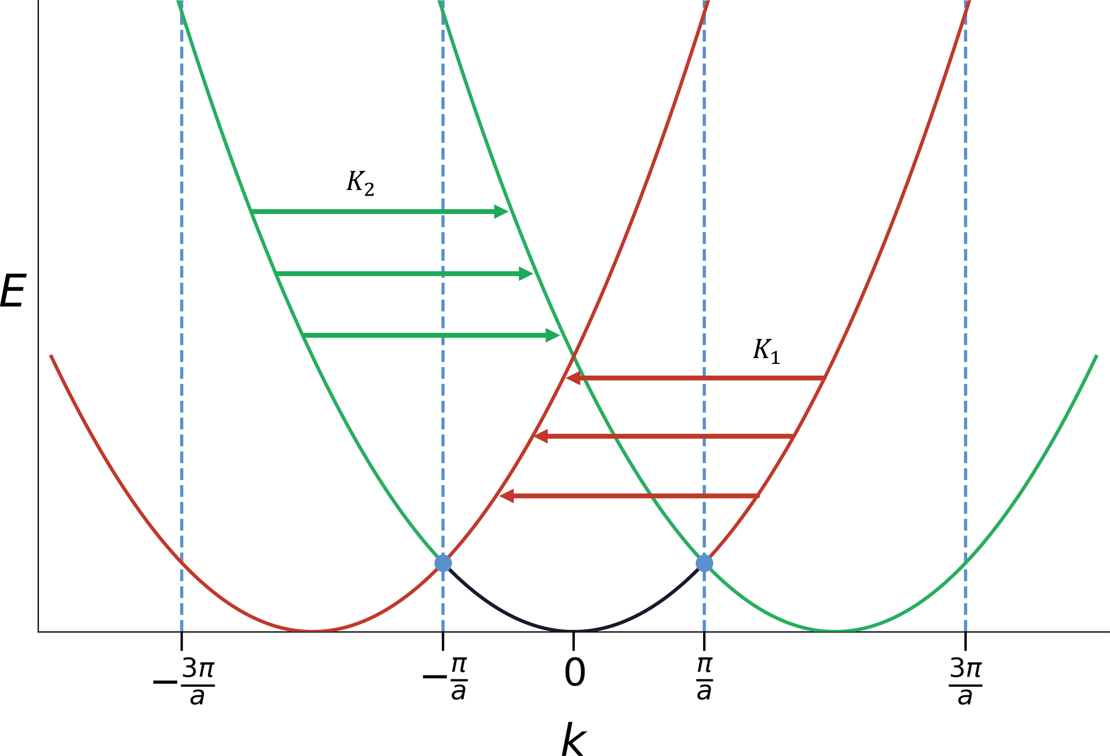
The black, red and green \(\epsilon(k)\) curves refer to three bands, with \(K = 0\), \(-K_1\) and \(K_2\), respectively.
\(K_1\) and \(K_2\) are both positive values, given the corresponding band in the figure and following the energy solution form presented above.
For all bands, we can choose to focus on the part inside the first Brillouin zone (BZ, \(-\pi/a \leq k \leq \pi/a\) in the 1D case presented above) and that is indeed how a band structure would usually be presented. Without the potential field, such a band structure is equivalent to the free electron case, which is the black parabola plotted in full. To see why, we can go back to the energy solution for, e.g., the red band,
\[\epsilon = \frac{\hbar^2(k + K_1)^2}{2m}\]which is nothing but the \(\epsilon = \frac{\hbar^2k^2}{2m}\) curve shifted left by \(K_1\). From the figure, we can clearly see that by such a shifting, the red part of the free electron dispersion (the \(\epsilon-k\) relation) is collapsed into the first BZ, reproducing identically the band corresponding to \(-K_1\) (again, in the first BZ).
-
With \(U = 0\), if we focus on the band labeled with \(\mathbf{K}\), then we know that only the coefficient \(c_{\mathbf{k} - \mathbf{K}_1}\) exists. All the other coefficients \(c_{\mathbf{k} - \mathbf{K}'}\) with \(\mathbf{K}' \neq \mathbf{K}_1\) does not exist, meaning that different bands are not impacting each other – the reason why we can reproduce the free electron case identically. As \(U\) becomes non-zero, we would expect coefficients \(c_{\mathbf{k} - \mathbf{K}'}\) with \(\mathbf{K}' \neq \mathbf{K}_1\) start to emerge, but we do expect them to be on the order of \(\mathbb{O}(U)\) (at least), i.e., as \(U\) vanishes, they should vanish.
-
Since \(U_{\mathbf{k} - \mathbf{K}}\) refers to the Fourier transform coefficients, they should be on the order of \(\mathbb{O}(U)\).
-
Regarding the Eqn. 9.13, the following statement is presented in Chapter-9,
Equation (9.13) asserts that weakly perturbed nondegenerate bands repel each other, for every level \(\epsilon_{\mathbf{k}-\mathbf{K}}^0\) that lies below \(\epsilon_{\mathbf{k}-\mathbf{K}_1}^0\) contributes a term in (9.13) that raises the value of \(\epsilon\), while every level that lies above \(\epsilon_{\mathbf{k}-\mathbf{K}_1}^0\) contributes a term that lowers the energy.
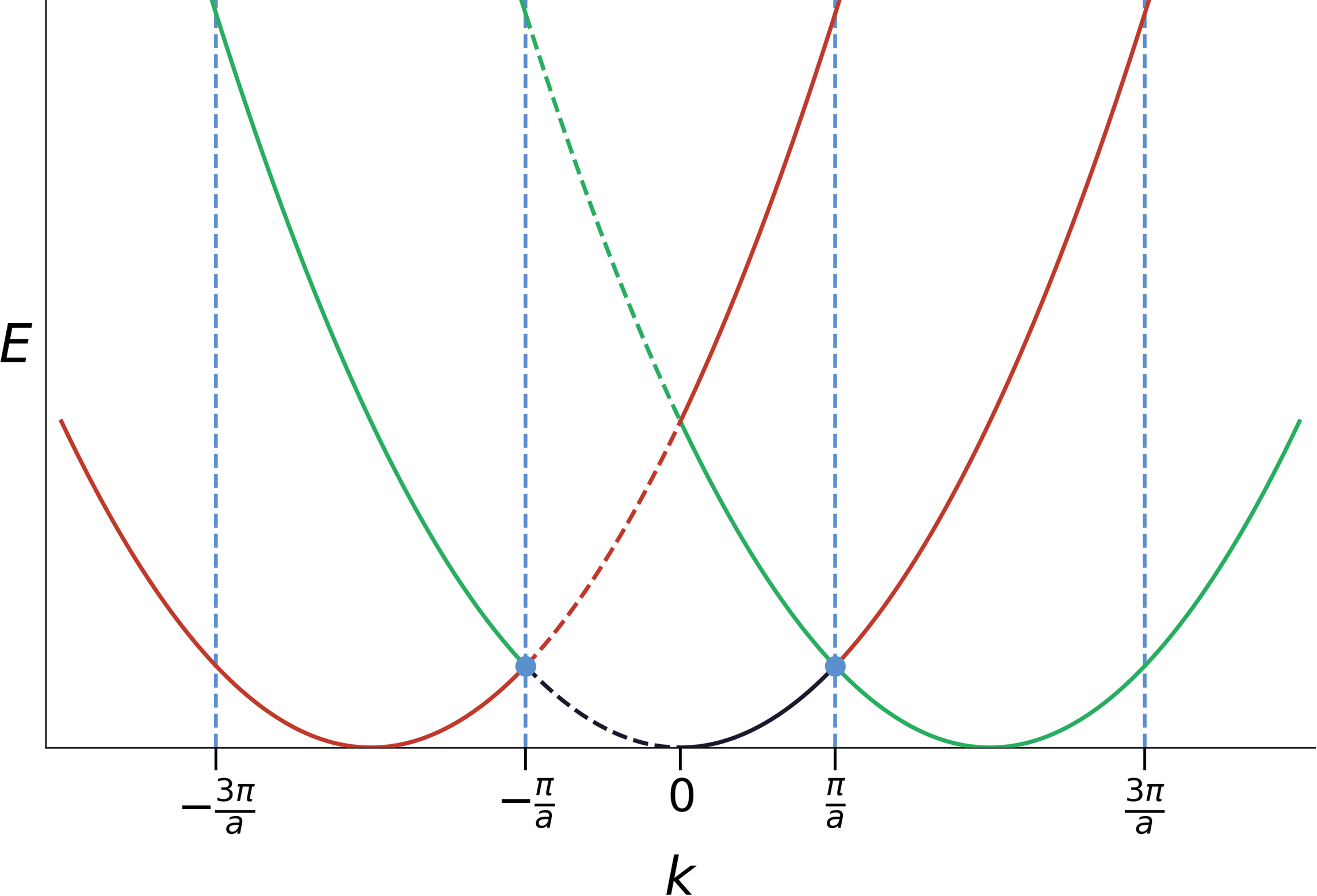
The diagram above demonstrates the point – for the dashed parts of bands, the red band sits between the black and green bands in the energy level. Therefore, when the potential becomes non-zero, the green one tries to push the red one down a bit while the black one triesd to push it up a bit.
-
Finally, we come to the point where the band gap emerges, at the BZ boundary. This originates from dealing with the degenerate case where multiple bands give the same energy. This is the part where the band structure is impacted the most significantly by the existence of the weak potential. Condition for the degeneracy coincides with the Bragg reflection condition. According to the energy solution presented above, the degeneracy means \(\vert \mathbf{k} \vert = \vert \mathbf{k} -\mathbf{K} \vert\)., which is exactly the Bragg reflection condition as presented below,
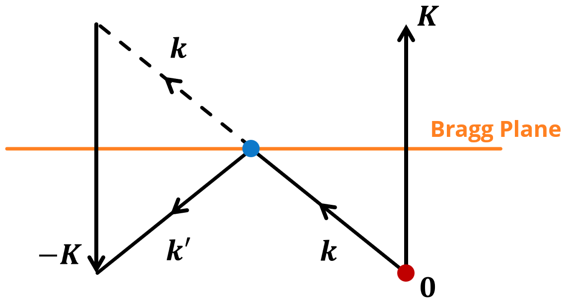
Two relevants notes about the coincidence of the degeneracy (thus the band gap emergence) and the Bragg reflection.
-
Given the Fourier expansion of the potential,
\[U(\mathbf{r}) = \sum_{\mathbf{K}} U_{\mathbf{K}}e^{i\mathbf{K} \cdot \mathbf{r}}\]the interaction matrix element of this potential between the incident (\(\mathbf{k}\)) and scattered (\(\mathbf{k}'\)) plane wave states can be given as,
\[\langle \mathbf{k}' \vert U \vert \mathbf{k} \rangle = \frac{1}{V} \int e^{-i\mathbf{k}'\cdot\mathbf{r}} \left( \sum_{\mathbf{K}} U_{\mathbf{K}}\, e^{i\mathbf{K}\cdot\mathbf{r}} \right) e^{i\mathbf{k}\cdot\mathbf{r}} \, d\mathbf{r} = \sum_{\mathbf{K}} U_{\mathbf{K}}\, \delta_{\mathbf{k}',\, \mathbf{k}+\mathbf{K}}\]That means, the periodic potential only connects states that differ by a reciprocal lattice vector \(\mathbf{K}\). This is just the Bragg’s law in quantum mechanics language.
-
Physical picture of the gap emergence. Taking the 1D case as an example, the electron density distribution corresponding to the two eigen states can be given as (see Eqn. 9.30 in Chapter-9),
\[\begin{align} \vert \psi_+(x)\vert^2 & \propto cos^2\bigg( \frac{\pi x}{a} \bigg)\\ \vert \psi_-(x)\vert^2 & \propto sin^2\bigg( \frac{\pi x}{a} \bigg) \end{align}\]where we can see that the dense region of electrons is located differently relative to where ions are located, for the two states. For the one with the electrons dense region coinciding with the ion position, the energy is expected to be lower (attraction by ion) and the other case will be with higher energy. This is the physical picture for the band gap emergence.
-
Filling bands with electrons
Say we havea finite crystal with \(N_1\times N_2 \times N_3\) primitive unit cells and pritimive lattice vectos \(\mathbf{a}_1\), \(\mathbf{a}_2\) and \(\mathbf{a}_3\). The total number of primitive unit cell is \(N = N_1N_2N_3\). Assuming we only have a single atom as the motif in the primitive unit cell, the total number of atoms is also \(N = N_1N_2N_3\). Given the Born-Von Karman (periodic) boundary condition, the wavefunction must obey,
\[\psi(\mathbf{r} + N_i\mathbf{a}_i) = \psi(\mathbf{r}), \quad i = 1, 2, 3\]Using Bloch’s theorem,
\[\begin{align} \psi_{n\mathbf{k}}(\mathbf{r} + N_i\mathbf{a}_i) & = e^{i\mathbf{k} \cdot (\mathbf{r} + N_i\mathbf{a}_i)}u_{n\mathbf{k}}(\mathbf{r} + N_i\mathbf{a}_i)\\ & = e^{i\mathbf{k} \cdot N_i\mathbf{a}_i} e^{i\mathbf{k} \cdot \mathbf{r}} u_{n\mathbf{k}}(\mathbf{r})\\ & = e^{i\mathbf{k} \cdot N_i\mathbf{a}_i} \psi_{n\mathbf{k}}(\mathbf{r}) \end{align}\]Accordingly, the boundary condition above requires,
\[e^{i\mathbf{k}\cdot N_i\mathbf{a}_i} = 1 \quad \Rightarrow \quad \mathbf{k}\cdot N_i\mathbf{a}_i = 2\pi \times \text{integer}\]Write \(\mathbf{k}\) in terms of reciprocal lattice basis vectors \(\mathbf{b}_1, \mathbf{b}_2, \mathbf{b}_3\) (defined by \(\mathbf{a}_i \cdot \mathbf{b}_j = 2\pi\delta_{ij}\)),
\[\mathbf{k} = \frac{m_1}{N_1}\mathbf{b}_1 + \frac{m_2}{N_2}\mathbf{b}_2 + \frac{m_3}{N_3}\mathbf{b}_3, \qquad m_i \in \mathbb{Z}\]Restricting to the first BZ only (band structure is periodic in reciprocal space and thus we only need to focus on the first BZ), the number of allowed \(\mathbf{k}\) values are \(N = N_1N_2N_3\), same as the total number of atoms. This is kind of expected – as we change from the real to reciprocal space, the total number of degrees of freedom should not change. Further, this means for each band, we have \(N = N_1N_2N_3\) allowed \(\mathbf{k}\) values. Therefore, the number of electrons that each band and host is \(2N\) – the Pauli exclusion principle allows only 2 electrons per \(\mathbf{k}\), namely spin up and down. Now, we can try to use the band structure to understand the conductivity. Let’s take the 1D case for simplicity – the 3D case is more realistic yet more complicated, and the 1D case can at least gives us a flavor so that we can touch and feel the principle. If the atom contains odd number of outer shell electrons, since each band can only host \(2N\) electrons, all electrons in this case tend to half fill the band (either half filling the first band for 1 outer shell electron case or half filling the second band for 3 outer shell electrons case, etc.), leaving the Fermi level right within the band so that electrons can be easily excited to travel freely, thus conducting. Elements with even number of outer shell electrons tends to be the other way round, with bands fully filled. Therefore, when gap opens up (as the result of the weak potential field, as discussed above), it always takes energy to bring electrons to the empty band (the conduction band, so they can travel freely), thus they tend to be insulating.
In 2D or 3D, the band structure is more complicated and the band filling is not as straightforward as it is for the 1D case. Regarding the energy level, the BZ boundary may be located within other bands, so even though the gap opens up at the BZ boundary, still it is possible that the Fermi level is located within a band. As such, the band gap at the BZ boundary does NOT make elements with even number of outer shell electrons insulating, like Mg.
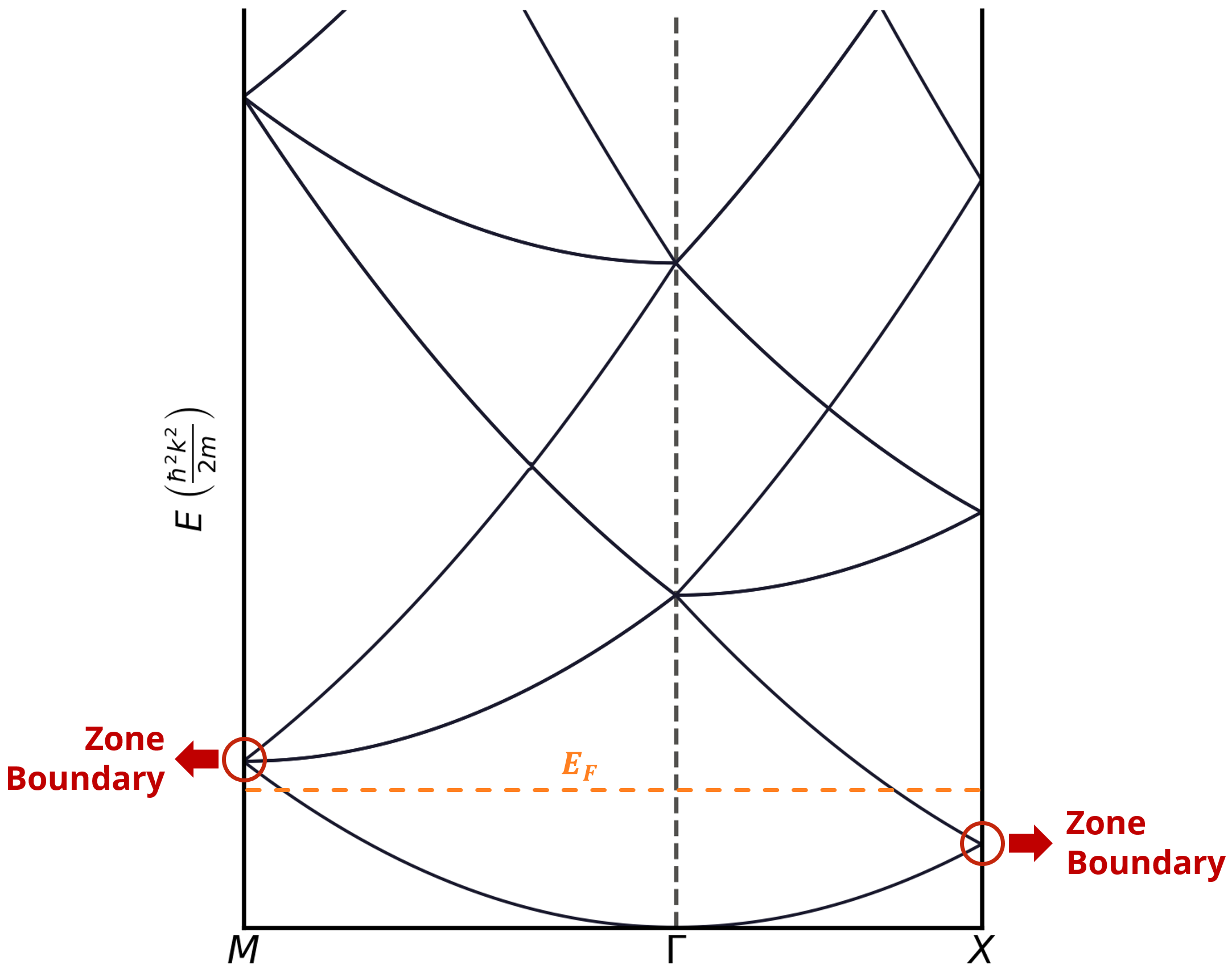
As shown in the figure above, given the Fermi level \(E_F\), the first \(\Gamma \rightarrow M\) band is still filling even when the first \(\Gamma \rightarrow X\) band is already full. Therefore, even a gap opens at the zone boundary \(X\), the Fermi level is still within a band (the first \(\Gamma \rightarrow M\) band), in which case we will still have a conductor. It is only when the gap at \(M\) opens wide enough so the whole first \(\Gamma \rightarrow M\) band is pushed below the Fermi level will we have an insulator.
Tight binding model
A very nice walkthrough of the tight binding model can be found in Ref. [4] by M. Roy, which I found is pretty much self-contained – just follow it and we should get a very good idea about how the tight binding model works. For earlier discussions in this post, we mainly base ourselves in the free electron model – we start from it and add in weak potential where they move in and we build up the band structure. In fact, the free electron model itself shows the band structure already, originating from the energy solution \(\epsilon = \hbar^2k^2/(2m)\). When collapsing regions beyond the first BZ all into the first BZ, the commonly seen band structure becomes clear. The tight binding model takes a bottom-up approach to build up the band structure. As mentioned at the very beginning of the post, in atoms, we have discrete energy levels. We then put atoms into a solid and we allow those atomic states to interact with each other. As shown in the tight binding framework, the energy levels will be broadened as the result of the interaction, giving rise to the band structure.
I am not planning to reiterate details in Ref. [4]. Instead, I will just put down several notes that I think will be helpful for understanding the material.
-
The single particle Hamiltonian is given as,
\[H = H_{\text{at}} + \Delta U\]where \(H_{\text{at}}\) is the hamiltonian for a single atom and \(\Delta U\) encodes
all the differences between the true potential in the crystal and the potential of an isolated atom. This is just a reiteration of the statement in Ref. [4] and here I just quoted the part that needs to be emphasized. -
When we say
\[\gamma(\vert \mathbf{R} \vert) = \int \phi^*_i(\mathbf{r}) H \phi_i(\mathbf{r} + \mathbf{R})\,d\mathbf{r}\]overlap integralin the context of tight binding model, we mean,between wavefunctions located on separate atomic sites (\(\mathbf{R} \neq 0\)) in the crystal. The
\[\int \phi_i^*(\mathbf{r})\phi_j(\mathbf{r}+\mathbf{R})\,d\mathbf{r} = \begin{cases} 1 & \text{if } i=j \text{ and } \mathbf{R}=0 \\ 0 & \text{otherwise.} \end{cases}\]direct overlapof atomic states across different lattice sites is given as, -
The building block of the tight binding model is writing the Bloch’s function as a linear combination of atomic orbitals,
\[\psi_{n\mathbf{k}}(\mathbf{r}) = \frac{1}{\sqrt{N}}\sum_{\mathbf{R}}e^{i\mathbf{k} \cdot \mathbf{R}} \phi_n(\mathbf{r} - \mathbf{R})\]where \(N\) is the number of lattice sites in the crystal and \(1/\sqrt{N}\) ensures the normalization of the Bloch state. In Ref, [4], the linear combination form is directly presented. In the node that I put in Ref. [4] (the exact PDF shared below, private access only), the we start from the general linear combination from and use the Bloch’s theorem to derive the linear combination coefficients. We can reproduce the exact form as presented above.
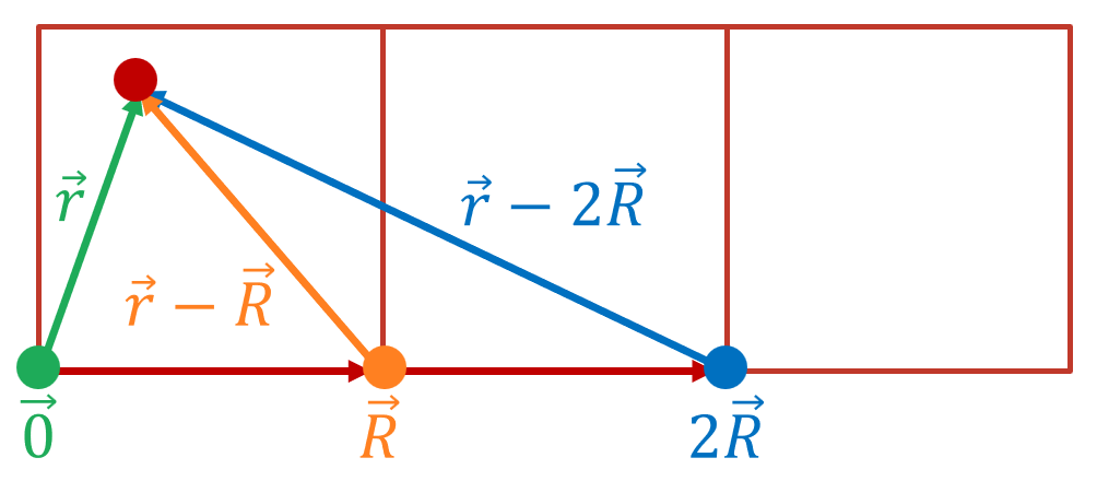
Shown in the figure is an illustration for the basic idea of the tight binding model. For any position \(\mathbf{r}\) (doesn’t have to be in the first cell), contributions to the Bloch’s wave function from atomic orbitals in various cells are illustrated in the figure. The \(\mathbf{r} - \mathbf{R}\) transforms the position \(\mathbf{r}\) to the local coordinate of cell \(\mathbf{R}\) – this is indeed the atomic state evaluated at \(\mathbf{r}\) with the atom located at \(\mathbf{R}\). Each contribution carries a ‘propagation’ factor, given as \(e^{i\mathbf{k} \cdot \mathbf{R}}\).
-
What is tight binding? In the tight binding model, ‘tight binding’ emphasizes the direct overlap being 0 and the overlap integral being small, among different lattice sites. So, atomic orbitals are pretty much staying local, i.e., tight binding to their own atoms.
Wannier function
Since the Bloch’s function is periodic in reciprocal space, it can be Fourier transformed to give,
\[\phi_{\mathbf{R}}(\mathbf{r}) = \frac{1}{N}\sum_{\mathbf{k}} e^{-i\mathbf{k} \cdot \mathbf{R}} \psi_{\mathbf{k}}(\mathbf{r})\]where
-
\(\mathbf{R}\) is the lattice vector. Therefore the Wannier function is a localized function attached to each of the Bravais lattice vector.
-
\(N\) is the number of pritimive cells in the crystal.
-
The sum is over \(\mathbf{k}\) in the first BZ. The space variable \(\mathbf{r}\) is not touched at all.
The orthogonality of Wannier functions for different lattice sites is proved in Ref. [5] and won’t be touched here. Basically, it means the set of Wannier functions can be used as a reliable basis set in the Hilbert space. The following property of the Wannier function is noteworthy,
\[\phi_{\mathbf{R}}(\mathbf{r}) = \phi_{\mathbf{R} + \mathbf{R}'}(\mathbf{r} + \mathbf{R}')\]Proof.
\[\begin{align} \phi_{\mathbf{R} + \mathbf{R}'} & = \sum_{\mathbf{k}} e^{-i\mathbf{k} \cdot (\mathbf{R} + \mathbf{R}')} \psi_{n\mathbf{k}}(\mathbf{r} + \mathbf{R}')\\ & = \sum_{\mathbf{k}} e^{-i\mathbf{k} \cdot (\mathbf{R} + \mathbf{R}')} e^{i\mathbf{k} \cdot \mathbf{R}'} \psi_{n\mathbf{k}}(\mathbf{r})\\ & = \sum_{\mathbf{k}} e^{-i \mathbf{k} \cdot \mathbf{R}} \psi_{n\mathbf{k}}(\mathbf{r})\\ & = \phi_{\mathbf{R}}(\mathbf{r}) \end{align}\]where we applied the following relation for Bloch’s function,
\[\psi_{n\mathbf{k}}(\mathbf{r} + \mathbf{R}') = e^{i\mathbf{k} \cdot \mathbf{R}'} \psi_{n\mathbf{k}}(\mathbf{r})\]which can be simply derived by putting \(\mathbf{r} + \mathbf{R}'\) into the Bloch’s function form, as given here.
Let \(\mathbf{R} = \mathbf{0}\), we obtain,
\[\phi_{\mathbf{0}}(\mathbf{r}) = \phi_{\mathbf{R}'}(\mathbf{r} + \mathbf{R}')\]This means for any lattice vector \(\mathbf{R}'\), the wavefunction evaluated at \(\mathbf{r} + \mathbf{R}'\) can always find its equivalent counterpart in cell \(\mathbf{0}\), evaluated at \(\mathbf{r}\). This is illustrated in the following figure,
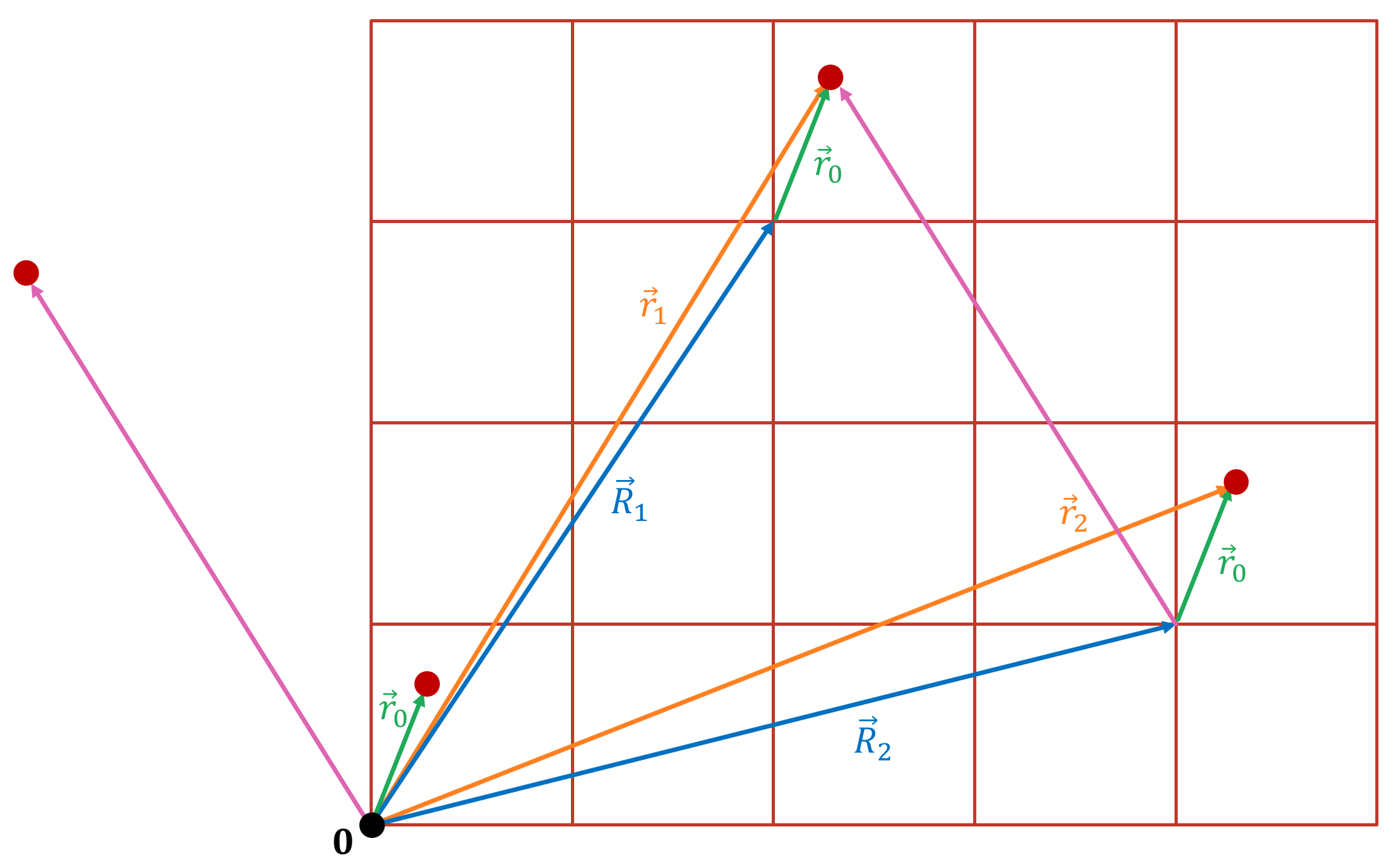
For \(\mathbf{r} = \mathbf{r}_1\) with the Wannier function at lattice vector \(\mathbf{R}_1\) and \(\mathbf{r} = \mathbf{r}_2\) with the Wannier function at lattice vector \(\mathbf{R}_2\), they are both equivalent to the evaluation of the Wannier function at \(\mathbf{r} = \mathbf{r}_0\). For the evaluation at \(\mathbf{r}_1\) with the Wannier function at \(\mathbf{R}_2\), the correspondingly equivalent spot with respect to the Wannier function at \(\mathbf{r} = \mathbf{r}_0\) is shown with the pinkish color.
References
[1] Neil W. Aschcroft and N. David Mermin, Solid State Physics, Harcourt College Publishers, 1976.
[2] Arthur P. Ramirez and Brian Skinner, Dawn of the Topological Age? Physics Today, September, 2020.
[3] Sommerfeld model.
[4] Tight binding model (my personal notion link, not public).
[5] Wannier function.