Learning Notes on Quantum Hall Effect

In this post, I am going to put down the learning notes for the lecture notes by Prof. David Tong [1].

Direction setup

See the figure on Wikipedia page here for all directions involved in the discussion.

The classical Hall effect

A particle of charge $-e$ in $\mathbf{B}=B\hat{z}$ moves in circles at the cyclotron frequency

:::info This can be derived with the motion equation,

or simply just follow the Newton’s equation,

\(evB = e\omega r B = mr\omega^2 \Rightarrow \omega = \frac{eB}{m}\) :::

The Drude model adds an electric field and friction,

In steady state ($d\mathbf{v}/dt = 0$), this gives,

Use $\mathbf{J} = -ne\,\mathbf{v}$, so $\mathbf{v} = -\mathbf{J}/(ne)$,

With $\mathbf{B}=B\hat{z}$, the cross product is $\mathbf{J}\times\mathbf{B} = (J_y B,\,-J_x B,\,0)$. Therefore,

Then we can write down the tensor form linking the electric field and the current,

This gives,

where,

The classical predictions are

Two observations. First, $\rho_{xy}$ doesn’t depend on $\tau$ and therefore it is nothing to do with the friction that electron feels (thus should be considered dissipationless). Second, $\rho_{xx}\to 0$ as $\tau\to\infty$ – as the friction disappears, the horizontal resistivity also disappears.

Actual observation

• Integer Hall effect (von Klitzing, 1980). The Hall resistivity forms plateaus at,

  \[\rho_{xy} = \frac{2\pi\hbar}{e^2}\frac{1}{\nu}, \ \ \ \ \nu\in\mathbb{Z},\]

  with $\rho_{xx}=0$ on each plateau and a spike in $\rho_{xx}$ between plateaus. Plateau centers sit at $B = n\Phi_0/\nu$, where the flux quantum is $\Phi_0 = 2\pi\hbar/e$.

• Disorder is essential. Adding disorder, but not too much, makes the plateaus more prominent. In a perfectly clean sample they are expected to vanish.

• Zero longitudinal resistivity. From $\sigma = \rho^{-1}$,

  \[\sigma_{xx} = \frac{\rho_{xx}}{\rho_{xx}^2 + \rho_{xy}^2}\]

  When $\rho_{xy}\neq 0$, $\rho_{xx}=0$ forces $\sigma_{xx}=0$. The sample acts like a perfect insulator and a perfect conductor at once. Below is included an illustration diagram,

  

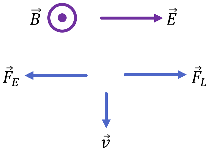
  In such a situation, the longitudinal current will be 0 – the current flows in the direction perfectly perpendicular to the applied electric field, due to the perfect balance between the electrostatic force and the Lorentz force, as shown in the diagram. Therefore, the longitudinal current being 0 is not because the resistivity is infinitely large – in fact, as given by the result above, the longitudinal resistivity is actually also 0. Instead, it is the result of the magnetic field.

Some Electrodynamics

Faraday’s experiments (moving a magnet through a coil, or varying a magnetic field near a loop) established that a changing magnetic flux through any closed loop induces an electromotive force (EMF, circulating electric field, 电动势) around that loop. Quantitatively,

where $C$ is any closed loop, $S$ is any open surface bounded by $C$. The minus sign is the physical content of Lenz’s law – the induced field opposes the change in flux. With Stokes’ theorem,

and further,

Accordingly we have,

Another equation from Maxwell’s is,

and also we have the following genuine result for any scalar field $f$ and any vector field $\mathbf V$,

Since we have $\nabla\cdot\mathbf B = 0$, from the genuine result presened above, we know that $\mathbf{B}$ can be written as,

which then automatically satisfies $\nabla\cdot\mathbf B=0$ for any choice of $\mathbf A$. Now plug $\mathbf B=\nabla\times\mathbf A$ into Faraday’s law,

where the last step just swaps the order of the (spatial) curl and the (temporal) partial derivative – since they act on independent variables and therefore the order does not matter. Rearranging,

By the first genuine result presented above, we know that $\mathbf E+\dot{\mathbf A}$ can be written as,

Landau level

Starting from the force on charged particle moving in the eletric and magnetic field,

and the fundamental results from electrodynamics presented in the previous section,

The Lagrangian \(L\) and the Hamiltonian for electrons moving in the magnetic field can be derived – refer to Ref. [2] (see §1.5). Tong’s book [1] directly lays out the result, based on which the quantization is carried out. The Hamiltonian is given as,

The quantized Hamiltonian (see Ref. [1] for details – §1.4) is shown to reproduce the one for a harmonic oscillator for which the discrete energy levels can be given as,

where \(\omega_B\) is the cyclotron frequency given on the very top of this post. The harmonic oscillator form can be seen from the classical Hamiltonian form. Take $\mathbf{A} = xB\hat{y}$, the classical Hamiltonian can be given as,

where,

Here we see the familiar form of the Hamiltonian for a harmonic oscillator (a classical spring) – the first term is the kinetic energy and the second term is the potential energy of the spring [3, 4]. It is just that the \(x\) value is shifted to the left by \(kl_B^2\). Since we take the form for $\mathbf{A} = xB\hat{y}$ along the \(y\) axis, the Hamiltonian in its classical form presented above does not contain any \(y\) components. Therefore, the eigen state can be written as,

where the \(y\)-contained part is basically a free-propagating plane wave. The full version of the wave function from §1.4 in Ref. [1] is reproduced here,

where \(H_n\) refers to the Hermite polynomials [5], and the first few orders are given below,

As mentioned earlier, the eigen values of energy is independent of \(k\) and therefore for each energy level (indexed with \(n\)), all the states with different \(k\) are degenerate. Suppose the material dimension is \(L_x\) by \(L_y\). Along the \(y\) direction, we already know that it is basically just a plane wave and according to the periodic boundary condition, we should have,

Therefore the interval between two adjacent allowed \(k\) values is \(2\pi/L_y\). Looking at the \(x\) direction, we have the wavefunction stripe (see below for what this means) centered at \(x_0 = -kl_B^2\) and for sure the stripe should be located inside the sample, so,

Now, we can calculate the degeneracy of each energy level (basically, how many values of \(k\) allowed for each level),

With \(l_B^2 = \hbar/eB\) and \(\Phi_0 = 2\pi\hbar/e\),

Since \(\Phi_0\) is defined as the flux quantum, the degeneracy here means the number of such quanta – the total flux \(AB\) divided by the flux quantum.

To see what we mean by ‘wavefunction stripe’ mentioned above, we can plot out the squared wavefunction,

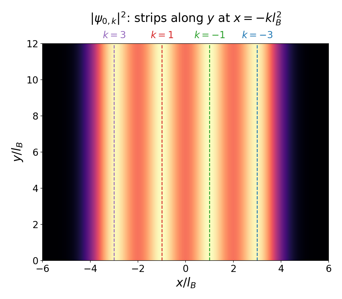
As expected, the distribution along the \(y\) direction is uniform and along the \(x\) direction, we have those stripes.

:::info Looking at the wavefunction solution given above and its visualization, we may be wondering where the circular motion. Since we are dealing with the situation where electrons are moving in a magnetic field, and we know that electrons should be making circular motion in the field. But it seems that we never saw such a circular feature in the wavefunction. What is happening? Several things. First, the wavefunction presented here are stationary so there is no time component at all. Therefore, indeed we should not be expecting any circular motion since there is no motion at all in the presented wavefunction – it is a time average. Second, the wavefunction is only the basis function corresponding to the Landau gauge ($\mathbf{A} = xB\hat{y}$). Since the basis function is gauge dependent anyhow, a single basis function does not represent anything physical. It is only the combination of those basis functions that will yield something physical. Indeed, if we consider all possible stripes altogether, we won’t have stripes at all since indeed physically, we should not be expecting any stripes in the physical setting – electrons moving in a uniform magnetic field. Third, if we calculate the current flow given the wavefunction solution, we should be able to see the circular feature. :::

Adding in the electric field, §1.4.2 in Ref. [1] shows the \(k\)-degeneracy is broken and the energy levels are given as,

Electrons drifts along the \(y\) direction as,

That is exactly the first diagram I presented earlier in the post.

Hall conductivity

The current in the $\nu$ filled Landau levels (charge times velocity, summed over all filled states),

With \(\mathbf{A} = xB\,\hat{\mathbf{y}}\), the two components are,

Each state is $\psi_{n,k} = e^{iky}f_n(x - x_0)$, with $f_n$ a real Hermite function centered at $x_0$.

Since $f_n$ is real,

No current flows along \(\mathbf{E}\). The \(y\) component of \(\boldsymbol{\pi}\) has two parts,

Since we know that the Hamiltonian reproduce the harmonic oscillator, the average \(x\) position should be the center of the oscillator. From the wavefunction form in Eqn. 1.20 in Ref. [1] (also presented earlier in this post – see the Landau level section) with electric field and the form in Eqn. 1.24 in Ref. [1] with the electric field, we can obtain the average position of the harmonic oscillator, as,

Substituting,

Back to the filled states summation earlier,

The term inside the summation is a constant so can be pulled out of the summation and therefore the whole summation is all about counting the number of states, which I have already presented earlier, namely \(AB/\Phi_0\). So,

Writing down the current density and link to the electric field, we can obtain the Hall conductivity tensor,

Edge mode

• The simple diagram shown in Fig. 14 illustrates the whole idea of the surface state, where the circular moving electrons are bounced by the boundary so that they just move along a single direction, opposite between two opposite boundaries.

• The opposite drifting velocity can be explained by the potential shape in Fig. 15, with the drifting velocity given as,

  \[v_y = -\frac{1}{eB}\frac{\partial V}{\partial x}\]

• Edge modes are chiral and they are immune to impurity since the one-way moving electrons are hard to disrupted.

Disorder and Plateaus

The filling factor is the density divided by the number of states per level per unit area,

For fixed $n$, $\nu$ is an integer only at the special fields $B = n\Phi_0/\nu$. At any other field, $\nu$ has a fractional part. For example, $\nu = 2.4$ means two full levels plus a third level that is 40% occupied. For fully filled level, every nearby state is occupied, the next empty state is $\hbar\omega_B$ away, and a weak field can’t move electrons across that gap. A partly filled level has occupied and empty states at the same energy, because the $AB/\Phi_0$ states in a level are degenerate. Any small perturbation, such as an impurity or a weak field, can move an electron into an empty state at no energy cost. That allows scattering and dissipation, so,

As for \(\sigma_{xy}\), it can always be argued that for a clean, translation-invariant sample, there always exists such a reference frame traveling at the drift velocity \(\mathbf{v} = \mathbf{E}\times\mathbf{B}/B^2\) where the electric field vanishes. When going back to the lab frame, the whole electron gas moves at $\mathbf{v}$, and therefore $\mathbf{J} = -ne\,\mathbf{v}$, giving,

:::info For $v \ll c$, the fields in a frame moving at velocity $\mathbf{v}$ are [6],

Choose $\mathbf{v} = \mathbf{E}\times\mathbf{B}/B^2$. Using $(\mathbf{a}\times\mathbf{b})\times\mathbf{c} = \mathbf{b}(\mathbf{a}\cdot\mathbf{c}) - \mathbf{a}(\mathbf{b}\cdot\mathbf{c})$ and $\mathbf{E}\perp\mathbf{B}$,

so $\mathbf{E}’ = 0$. :::

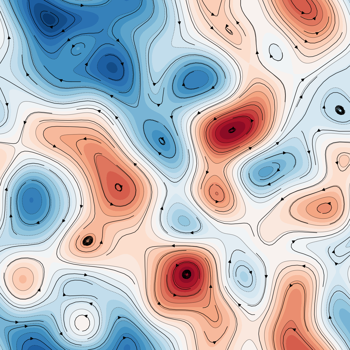
So, in a perfectly clean material, the Hall conductivity just shows a continuous variation as \(B\) varies and we are not yet seeing any plateaus behavior. What we are missing is the consideration of disorder. The existence of disorder in pratical materials give rise to random potential and Ref. [1] shows that electron orbit centers drift along equipotentials (the contour levels along which the random potentials are equal – see the diagram below).

Now, the physical picture for the emergence of the plateaus is like this. First, the existence of disorder in the system will broaden the Landau levels, as shown in Fig. 17 in Ref. [1]. The broadened Landau level is given as,

:::info Here it is assumed that the random potential is pretty much localized and around each orbit center of electrons, it can be regarded as constant (and therefore can be directly added to the energy eigen value for the energy levels). :::

If we write,

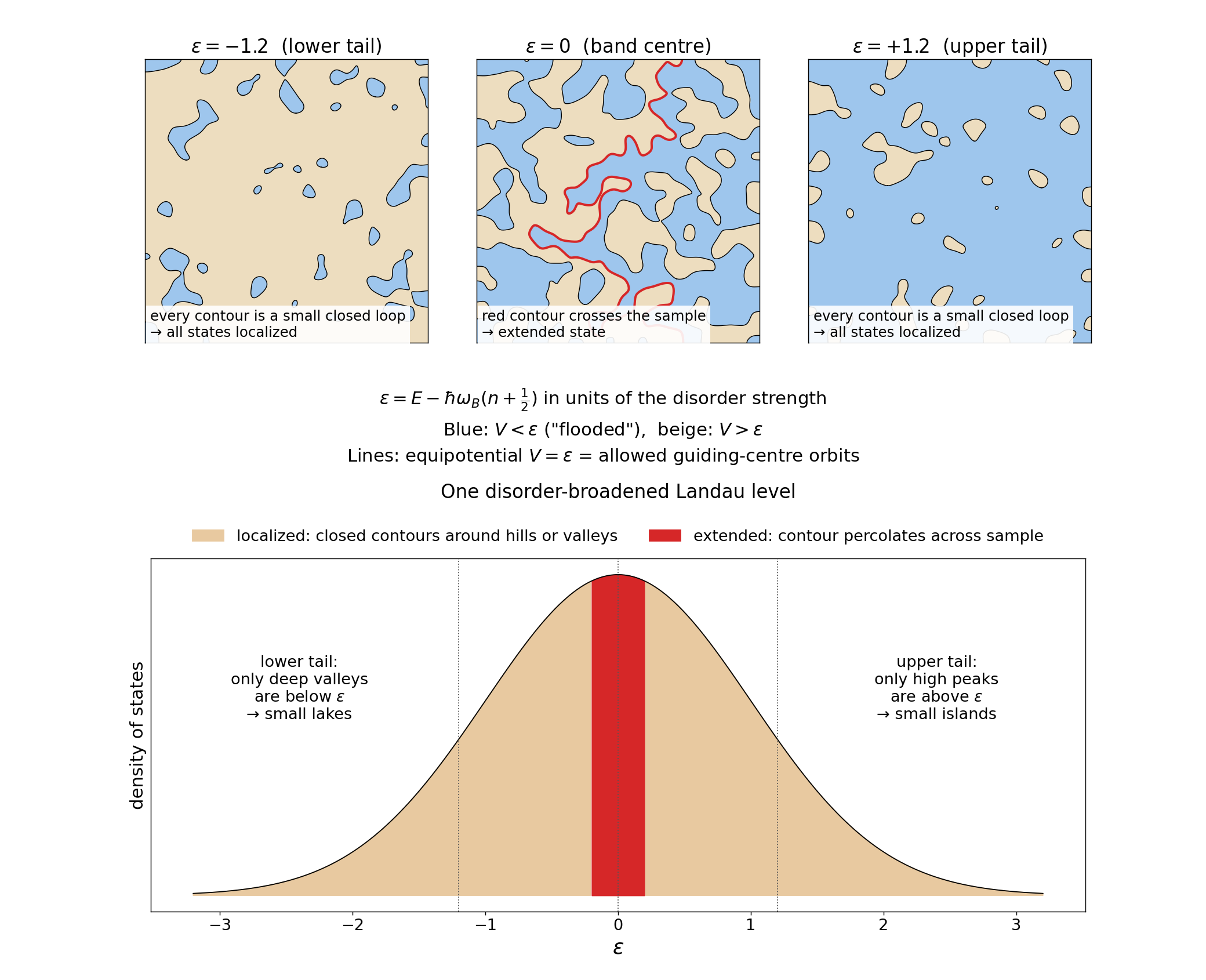
The orbit center must then stay on the equipotential $V(X,Y) = \epsilon$. Imagine the random potential as a landscape, filled with water up to height $\epsilon$. The shoreline is exactly the contour $V = \epsilon$, so it traces the orbits allowed at that energy.

Here below is presented a metaphor to understand the situation,

• Lower tail, $\epsilon = -1.2$ (left panel). The water level is low, so only the deepest valleys hold water. The result is small, separate lakes, each with a short closed shoreline. An electron at this energy circles one lake forever, so the state is localized.

• Upper tail, $\epsilon = +1.2$ (right panel). The water level is high and almost everything is flooded. Only the highest peaks stick out as small islands. Each shoreline is again a short closed loop around one island, so the state is localized.

• Band center, $\epsilon = 0$ (middle panel). Land and water each cover about half the area, and both form large, winding, connected regions. The shoreline between them can run all the way across the sample (red line). An electron on it travels from one side to the other, so the state is extended and can carry current.

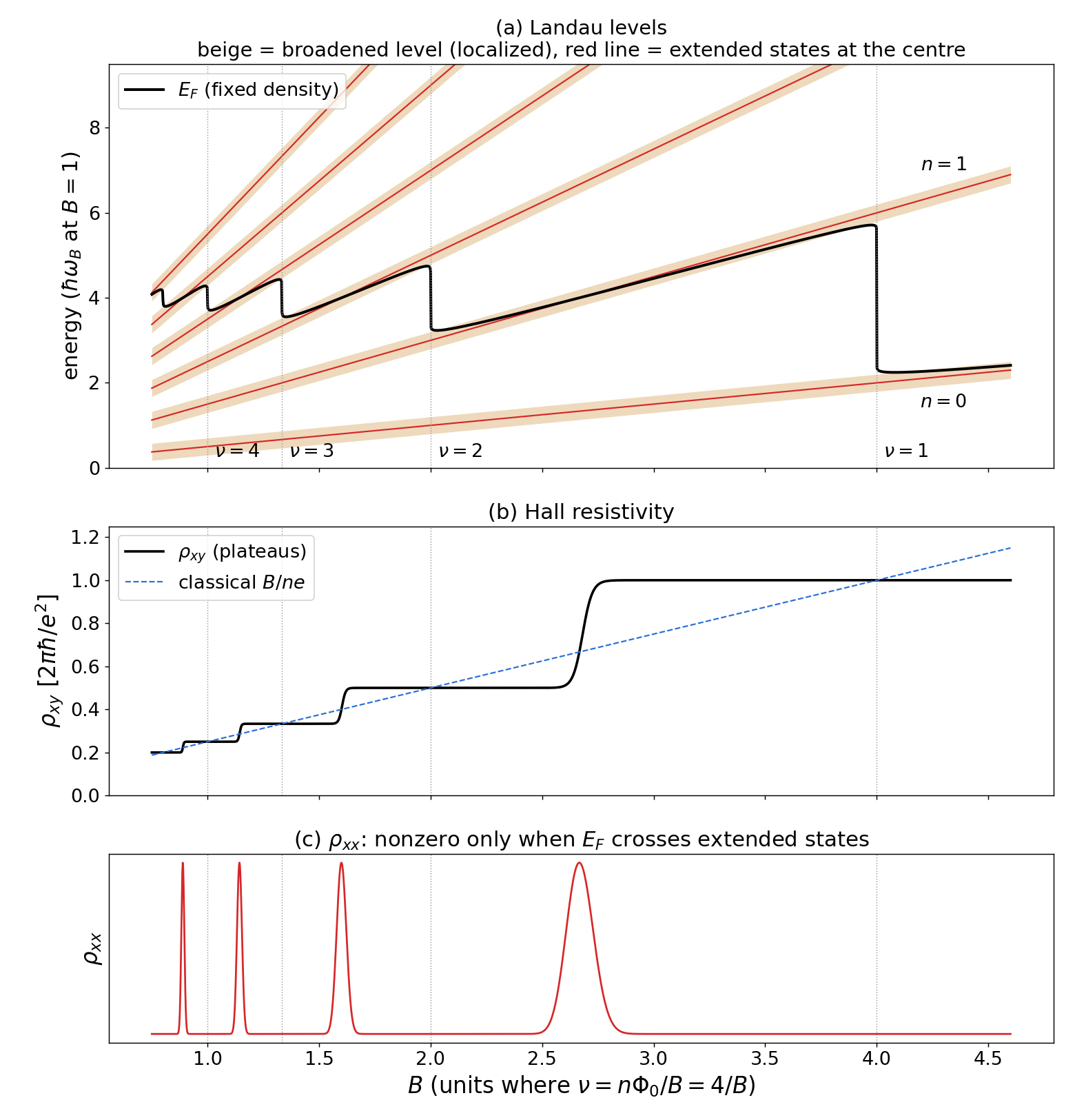
As $B$ changes,

• Level energy changes – $E_n = \hbar\omega_B\left(n+\tfrac{1}{2}\right)$, with $\omega_B = eB/m$. Every level rises in proportion to $B$, which is the tilted red lines in panel (a).

• States per level change – $B/\Phi_0$ per unit area, also proportional to $B$.

The filling factor is,

As $B$ increases, $\nu$ decreases continuously. Each level holds more electrons, so electrons occupying top levels will shift to to the lower levels, and accordingly the high level occupation drops from 1 toward 0. $E_F$ therefore moves down through that level’s density of states – first the upper tail, then the center, then the lower tail. When the fraction reaches 0, the level is empty. $E_F$ then crosses the gap, and lands at the top of the next level down, which is now full. Then the process repeats. In panel (a), the black $E_F$ curve follows one level (beige band) upward, sliding down relative to it, then drops to the next level at the vertical jumps near integer $\nu$. Most of the time, $E_F$ is in the beige localized tails, and accordingly the electrons being added or removed go into localized states, carrying no current. So $\sigma_{xx} = 0$, and $\rho_{xy}$ stays at the value set by the full levels below. These are the flat plateaus in panel (b). Only when $E_F$ passes the red line at a level’s center do extended states change occupation. There $\rho_{xx}$ spikes (panel c) and $\rho_{xy}$ steps to the next plateau. Comparing the classical line $\rho_{xy} = B/ne$ (dashed in panel b), we can see the plateaus cross it near integer $\nu$, where the calculation with filled levels applies exactly.

References

[1] Quantum Hall Effect

[2] H. Goldstein, C. Poole, J. Safko, Classical Mechanics, 3rd ed.

[3] Hamiltonian Mechanics Examples

[4] Simple Harmonic Oscillator

[5] Hermite polynomials

[6] J. D. Jackson, Classical Electrodynamics, 3rd ed. (Wiley, 1999)